
If you’ve been following the arXiv, or keeping abreast of developments in high-energy theory more broadly, you may have noticed that the longstanding black hole information paradox seems to have entered a new phase, instigated by a pair of papers [1,2] that appeared simultaneously in the summer of 2019. Over 200 subsequent papers have since appeared on the subject of “islands”—subleading saddles in the gravitational path integral that enable one to compute the Page curve, the signature of unitary black hole evaporation. Due to my skepticism towards certain aspects of these constructions (which I’ll come to below), my brain has largely rebelled against boarding this particular hype train. However, I was recently asked to explain them at the HET group seminar here at Nordita, which provided the opportunity (read: forced me) to prepare a general overview of what it’s all about. Given the wide interest and positive response to the talk, I’ve converted it into the present post to make it publicly available.
Well, most of it: during the talk I spent some time introducing black hole thermodynamics and the information paradox. Since I’ve written about these topics at length already, I’ll simply refer you to those posts for more background information. If you’re not already familiar with firewalls, I suggest reading them first before continuing. It’s ok, I’ll wait.
Done? Great; let me summarize the pre-island state of affairs with the following two images, which I took from the post-island review [3] (also worth a read):

On the left is the Penrose diagram for an evaporating black hole in asymptotically Minkowski space. We suppose the black hole formed from some initially pure state of matter (in this case, a star, denoted in yellow), and evaporates completely via the production of Hawking radiation (represented by the pairs of squiggly lines). The key thing to note is that the Hawking modes are pairwise entangled: the interior partner is trapped behind the horizon and eventually hits the singularity, while the exterior partner is free to escape to infinity as Hawking radiation. An observer who remains far outside the black hole and attempts to collect this radiation will then find the final state to be highly mixed (in fact, almost thermal), since along any timeslice (the green slices), she only has access to the modes outside the horizon. But since we took the initial state to be pure (entropy 
The evaporation process is depicted in the right figure, which schematically plots various relevant entropies over time. On the one hand, the Bekenstein-Hawking entropy of the black hole starts at some large value given by the surface area, and steadily decreases as the hole evaporates (orange curve). Meanwhile, the entropy of the radiation starts at zero, and then steadily increases over time as more and more modes are collected. This is the result given in Hawking’s original calculation [4], represented by the green curve. The expectation from unitarity is that the entropy of the radiation should instead follow the so-called Page curve, shown in purple. The idea is that at around the halfway point — more accurately, the point at which the entropy of the radiation equals the entropy of the horizon — the emitted modes start to purify the previously-collected radiation, so the entropy starts to decrease. Eventually, when the black hole has completely evaporated and all the “information” has been emitted, the radiation should again be in a pure state with
In a nutshell, the island formula is a prescription for computing the entropy of the radiation in such a way as to reproduce the Page curve. The claim is that instead of naïvely tracing-out the black hole interior, one should assign the radiation the generalized entropy
![\displaystyle S_\mathrm{rad}=\mathrm{min}_\mathcal{X}\left\{\mathrm{ext}_\mathcal{X}\left[\frac{A(\mathcal{X})}{4G_N}+S_\mathrm{semi-cl}\left(\Sigma_\mathrm{rad}\cup\Sigma_\mathrm{island}\right)\right]\right\}~, \ \ \ \ \ (1)](https://s0.wp.com/latex.php?latex=%5Cdisplaystyle+S_%5Cmathrm%7Brad%7D%3D%5Cmathrm%7Bmin%7D_%5Cmathcal%7BX%7D%5Cleft%5C%7B%5Cmathrm%7Bext%7D_%5Cmathcal%7BX%7D%5Cleft%5B%5Cfrac%7BA%28%5Cmathcal%7BX%7D%29%7D%7B4G_N%7D%2BS_%5Cmathrm%7Bsemi-cl%7D%5Cleft%28%5CSigma_%5Cmathrm%7Brad%7D%5Ccup%5CSigma_%5Cmathrm%7Bisland%7D%5Cright%29%5Cright%5D%5Cright%5C%7D%7E%2C+%5C+%5C+%5C+%5C+%5C+%281%29&bg=ffffff&fg=000000&s=0&c=20201002)
where 


Quantum Extremal Surfaces
While the Penrose diagram above (and most of those below) depicts a black hole in asymptotically flat space, the island formula (1) is properly formulated in AdS/CFT, which is where our story begins. In the interest of making this maximally accessible, let’s start at the beginning with my favourite picture of the hyperbolic disc, courtesy of M. C. Escher:
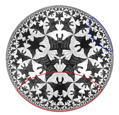
Here we have a gravitational theory living in the bulk anti-de Sitter (AdS) space, which is dual to some conformal field theory (CFT) living on the asymptotic boundary. (Since this picture is necessarily embedded in flat space, the hyperbolic nature of the bulk manifests in the fact that the devils are all the same size). Inherent in the nature of a duality is that every element on one side has an equivalent element on the other, and a major research area in AdS/CFT is completing the so-called holographic dictionary that relates them. One of the major lessons of the past decade is that entanglement entropy appears to play a significant role in this mapping. In particular, the Ryu-Takayanagi formula [5] states that the von Neumann entropy of a boundary subregion — e.g., the blue or red boundary segments I’ve drawn over the image above — is given by the area of the co-dimension 2 minimal surface in the bulk anchored to the boundary of said region that satisfies the homology constraint (see below) — e.g., the blue or red arcs extending towards the center — called the Ryu-Takayanagi or RT surface. More generally, the idea is that all of the physics within the enclosed bulk region can be described by operators living in the corresponding boundary segment (more precisely, its causal domain of dependence).
The most salient aspect of this proposal for our purposes is that it has precisely the same form as the Bekenstein-Hawking entropy, i.e.,

where 


where for consistency I’ve denoted the entropy of the radiation
Formally, the generalized entropy (3) is exactly the quantity that appears in the innermost brackets in the island formula (1), subject to the details of how one selects what semi-classical entropy to compute—more on this below. What about the 
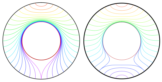
This is again the hyperbolic disc, but with a large AdS black hole whose horizon is demarcated by the inner circle. Now imagine starting with a small boundary subregion at the top of the image, whose corresponding bulk RT surface is drawn in red. As we make this region progressively larger, the RT surface lies deeper and deeper into the bulk—this is represented by the shading from red towards violet. Since the surfaces are defined geometrically, they are sensitive to the presence of the black hole, and get deformed around it as we include more and more of the boundary in the subregion under consideration. Eventually the subregion includes the entire boundary, and the corresponding RT surface is the violet one in the left image. For BTZ black holes, that’s it.
In higher dimensions however, there’s a second RT surface that becomes relevant when the subregion reaches a certain size. Consider the right image, at the point where the RT surface for the subregion is blue. The old solution is the RT surface that loops back around the black hole, on the same side as the boundary subregion. The new solution is the RT surface that connects these same two boundary points on the opposite (that is, lower) side of the black hole, plus a piece that wraps around the horizon itself. The horizon is included because the RT prescription requires the surface to be homologous to the boundary (crudely speaking, we wrap a second piece around the black hole in order to excise the hole from the manifold, so that the solution remains in the same homology class. The fact that one must consider disconnected surfaces may seem rather bizarre, but there’s nothing intrinsically pathological about it; see [7] for more discussion and additional references on the homology constraint in this context). One can see visually that when the boundary subregion reaches a certain size, the combined length of these two pieces will be smaller than the length of the old RT surface that has to go around the black hole the long way. A priori, we now have an ambiguity in which bulk entity we identify with the entropy of the boundary subregion, which is resolved by the requirement that we choose the minimum among all such choices. (While I’m unaware of a satisfactory physical explanation for this, it appears necessary in order for the generalized entropy to satisfy subadditivity [8]). Therefore, as the size of the boundary subregion is continuously increased, a discontinuous (i.e., non-perturbative) switchover occurs to the new minimal surface. As we shall see, a similar switchover plays a crucial role in the island computation of the Page curve.
Now, a quantum extremal surface (QES) is a seemingly mild correction to the above prescription, whereby the semi-classical contribution is taken into account when selecting the surface itself. That is, in the above RT prescription, we selected the minimal surface (which fixes the area term in (3)), and then added the entropy of all the matter fields living between that fixed surface and the boundary (the second term in (3)). As argued in [9] however, the correct procedure is to instead find the surface such that the combination of both terms is extremized, which defines the QES, denoted 


In most cases, the difference between the QES and its classical counterpart is relatively small. However, the remarkable feature uncovered in [1,2] is that this can sometimes be quite large, and furthermore, that the QES can sometimes lie deep inside the black hole. This is in sharp contrast to the classical RT surfaces discussed above: as one can see in those rainbow images from [7], they never reach beyond the horizon. (In fact, this appears to be a limitation of all such classical probes, as my colleagues and I analyzed in detail when I was a PhD student [10]: one can get exponentially close to the horizon in some cases, but no better. The corresponding “holographic shadows” seem to represent a puzzle for holographers, since — as per AdS/CFT being a duality — the boundary must have a complete and equivalent description of the physics in the bulk, including the black hole).
These two elements — the minimality requirement, and the ability of QESs to probe behind horizons — are the key to islands.
Some Flat Space Intuition
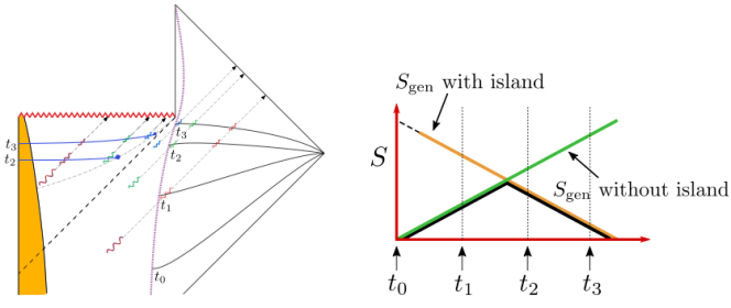
Let us set holography aside for the moment, and return to the flat space Penrose diagram for an evaporating black hole we introduced above. The review [3] does a great job painting an intuitive picture of how the QES changes the story. In particular, the various ingredients in (1) are shown in the following Penrose diagram:

The basic idea is as follows: suppose one is an external observer moving along the timelike trajectory given by the dashed purple line, who collects Hawking radiation that escapes to infinity. The latter comprises the semi-classical entropy along 
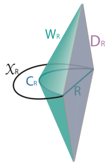
To understand why this QES appears, consider the following diagram, again from [3]. Suppose we fix a Cauchy slice at some point in the evaporation process (say, time 

If we repeat this process along an earlier Cauchy slice however, the picture is quite different. Before any radiation has been emitted, shrinking
We thus have two possible choices for the QES 


Shortly after the black hole starts to evaporate however, the second, non-vanishing QES appears some distance inside the horizon. The corresponding area contribution is initially very large, but steadily decreases as the hole evaporates. Crucially, the semi-classical contribution also declines, since we count modes in the union 
Since we’re instructed to always use the minimum QES, a switchover analogous to that we discussed in the context of RT surfaces thus occurs at the Page time: at this point, the area of the non-empty QES (which dominates over the corresponding semi-classical contribution) equals the semi-classical contribution from the empty QES. We therefore follow the black curve in the plot, which is the sought-after Page curve, where the change from an increasing (green) to decreasing (orange) entropy corresponds to a non-perturbative shift in the location of the minimal QES. In this way, the island formula obtains a result for the generalized entropy consistent with our expectations from unitarity.
However, while the exposition above paints a nice intuitive picture, it’s ultimately just a cartoon, and leaves many physical aspects unexplained—for example, how the interior “island” is able to purify the radiation, or the dependence of (the location of)
Just drink the Kool-Aid
There are two main stumbling blocks that must be overcome for the picture we’ve painted above to work:
- Large black holes in AdS don’t evaporate.
- The identification of the island with the radiation is ultimately imposed by hand.
The first of these is due to the fact that large AdS black holes, unlike their flat-space counterparts, are microcanonically stable: they have 

To circumvent this, [1,2] coupled the system to an auxiliary reservoir in order to force the black hole to evaporate. This is illustrated by the following figure from [2], in which a coupling between the asymptotic boundary and a previously-independent CFT that acts as a bath is turned on at the time indicated by the orange dot. Prior to this, radiation from the AdS
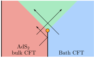
This is approximately the point at which I get off the metaphorical train. In particular, insofar as AdS/CFT is a duality between equivalent descriptions of the same system, not two systems that interact at some physical boundary, the so-called “absorbing boundary conditions” [1,2] claim when performing this operation do not appear to me to be valid. Another way to express this underlying point is that it is incorrect to treat the bulk and boundary as akin to tensor factorizations of a single all-encompassing Hilbert space. Rather, the radiation — which carries some finite energy — has an equivalent description in the boundary CFT. Allowing it to propagate into the boundary simultaneously decreases the energy of the bulk while increasing the energy of the boundary, thereby breaking the duality. Following the initial works above, an interesting attempt was made in [13] to make this construction more plausible by allowing the auxiliary system itself to be holographic. However, while the resulting “double holography” model is more technically refined, it ultimately still features fields propagating between different sides of the duality, so does not actually overcome the fundamental objection above.
Suppose however that one accepts such forced-evaporation models for the sake of argument—after all, the entire point of a toy model is to grant a sufficient deviation from reality that calculations become tractable (the tricky bit, and the focus of my skepticism here, lies in determining how much physics is retained in the result). One then has to contend with the second roadblock, namely identifying the radiation — now contained in the auxiliary reservoir — with the interior island. That is, when we wrote down the island formula (1), the semi-classical term was defined as the entropy over the union
Proponents of the island prescription would disagree with this claim. The review [3] for example addresses it explicitly as follows:
“Now a skeptic would say: `Ah, all you have done is to include the interior region. As I have always been saying, if you include the interior region you get a pure state,’ or `This is only an accounting trick.’ But we did not include the interior `by hand’. The fine-grained entropy formula is derived from the gravitational path integral through a method conceptually similar to the derivation of the black hole entropy by Gibbons and Hawking…”
The calculation they refer to is the replica trick for computing entanglement entropy, which I’ve written about before. And indeed, at least two papers [11,12] have claimed to derive the island formula via precisely such a replica wormhole calculation. The underlying idea is actually rather beautiful: the switchover to the new QES corresponds to an initially sub-leading saddlepoint in the gravitational path integral which becomes dominant at the Page time. (There’s a pedagogically exemplary talk on YouTube by Douglas Stanford in which he explains how this comes about in the toy model of [11]). The issue here is not that there’s anything wrong with the technical aspects of the above derivations per se. However, as I’ve stressed before, the conclusions one can draw from any derivation are dependent on the assumptions that go into it. In this case, the key assumption is that when sewing the replicas together, we make a cut along what becomes the island. That is, when we perform the replica trick, we make 

In derivations of the island formula, one makes a disjoint cut along
A proponent might argue that there are good reasons to join the replicas in this fashion; but producing the correct answer a posteriori should not be one of them. In short, my unfashionable opinion is that the claim in [12] that “[t]his new saddle suggests that we should think of the inside of the black hole as a subsystem of the outgoing Hawking radiation” is, at least at this point in our collective explorations/explanations, backwards: rather, if you think of the inside of the black hole as a subsystem of the outgoing Hawking radiation, you will get a new saddle. The logic works both ways in principle, I’m simply not quite convinced that we’ve justified running it in the popular direction.
Even if the island prescription is (ontologically) correct — and it may well be — it does not suffice to resolve the firewall paradox, for several reasons. Physically, it does not explain how the radiation is purified from an operational perspective, i.e., how unitarity is restored from a pure bulk entropy calculation (e.g., in Minkowski space without any bells and whistles). Additionally, it does not explain where Hawking’s original calculation [4] went wrong. Abstractly, one would say that the error is that he did not include this sub-leading saddle, which arises from the different ways of connecting the replica geometries. But insofar as Hawking’s calculation does not employ a gravitational path integral at all, an interesting open question that would likely shed light on the underlying physics of the island prescription is how to bridge the conceptual gap between the calculation via replica wormholes and the more down-to-earth calculation via Bogolyubov coefficients in the black hole scattering matrix.
To be sure, this is still a very interesting and non-trivial result. It’s remarkable that the bulk gravitational path integral includes these crucial replica wormhole geometries, despite the fact that the
References
- G. Penington, “Entanglement Wedge Reconstruction and the Information Paradox,” JHEP 09 (2020) 002, arXiv:1905.08255.
- A. Almheiri, N. Engelhardt, D. Marolf, and H. Maxfield, “The entropy of bulk quantum fields and the entanglement wedge of an evaporating black hole,” JHEP 12 (2019) 063, arXiv:1905.08762.
- A. Almheiri, T. Hartman, J. Maldacena, E. Shaghoulian, and A. Tajdini, “The entropy of Hawking radiation,” arXiv:2006.06872.
- S. W. Hawking, “Breakdown of predictability in gravitational collapse,” Phys. Rev. D 14 (Nov, 1976) 2460–2473.
- S. Ryu and T. Takayanagi, “Holographic derivation of entanglement entropy from AdS/CFT,” Phys. Rev. Lett. 96 (2006) 181602, arXiv:hep-th/0603001.
- T. Faulkner, A. Lewkowycz, and J. Maldacena, “Quantum corrections to holographic entanglement entropy,” JHEP 11 (2013) 074, arXiv:1307.2892.
- V. E. Hubeny, H. Maxfield, M. Rangamani, and E. Tonni, “Holographic entanglement plateaux,” JHEP 08 (2013) 092, arXiv:1306.4004.
- M. Headrick and T. Takayanagi, “A Holographic proof of the strong subadditivity of entanglement entropy,” Phys. Rev. D 76 (2007) 106013, arXiv:0704.3719.
- N. Engelhardt and A. C. Wall, “Quantum Extremal Surfaces: Holographic Entanglement Entropy beyond the Classical Regime,” JHEP 01 (2015) 073, arXiv:1408.3203.
- B. Freivogel, R. Jefferson, L. Kabir, B. Mosk, and I.-S. Yang, “Casting Shadows on Holographic Reconstruction,” Phys. Rev. D 91 no. 8, (2015) 086013, arXiv:1412.5175.
- G. Penington, S. H. Shenker, D. Stanford, and Z. Yang, “Replica wormholes and the black hole interior,” arXiv:1911.11977.
- A. Almheiri, T. Hartman, J. Maldacena, E. Shaghoulian, and A. Tajdini, “Replica Wormholes and the Entropy of Hawking Radiation,” JHEP 05 (2020) 013, arXiv:1911.12333.
- A. Almheiri, R. Mahajan, J. Maldacena, and Y. Zhao, “The Page curve of Hawking radiation from semiclassical geometry,” JHEP 03 (2020) 149, arXiv:1908.10996.
- P. Calabrese and J. Cardy, “Entanglement entropy and conformal field theory,” J. Phys. A 42 (2009) 504005, arXiv:0905.4013.
- D. Marolf and H. Maxfield, “Transcending the ensemble: baby universes, spacetime wormholes, and the order and disorder of black hole information,” JHEP 08 (2020) 044, arXiv:2002.08950
- R. Jefferson, “Comments on black hole interiors and modular inclusions,” SciPost Phys. 6 no. 4, (2019) 042, arXiv:1811.08900.
- R. Jefferson, “Black holes and quantum entanglement,” arXiv:1901.01149.
- E. Witten, “Gravity and the crossed product,” JHEP 10 (2022) 008, arXiv:2112.12828.
 in
in  -dimensional Minkowski (i.e., flat) spacetime. From
 ,
,  , and the creation/annihilation operators satisfy the standard equal-time commutation relation, which in our convention is
 ![{\big[a_k,a_{k'}^\dagger\big]=4\pi\omega\delta(\mathbf{k}-\mathbf{k}')}](https://s0.wp.com/latex.php?latex=%7B%5Cbig%5Ba_k%2Ca_%7Bk%27%7D%5E%5Cdagger%5Cbig%5D%3D4%5Cpi%5Comega%5Cdelta%28%5Cmathbf%7Bk%7D-%5Cmathbf%7Bk%7D%27%29%7D&bg=ffffff&fg=000000&s=0&c=20201002) , with the vacuum state
, with the vacuum state  such that
  . (The derivation of this commutation relation, as well as the reason for splitting the normalization in this particular way when identifying the modes
  , will be discussed below). Typically, we choose the positive solution to the Klein-Gordon equation,
  , so that the operator
  has an interpretation as the creation operator for a positive-frequency mode traveling forwards in time. Note however that this statement depends on the existence of a global timelike Killing vector. That is, the modes
  are of positive frequency with respect to some time parameter
  , by which we mean they’re eigenfunctions of the operator
  with eigenvalue

 , i.e.,
  . Since both sets of modes are complete, they must be linear combinations of one another, i.e.,
 ,
,  are called Bogolyubov coefficients. (Note that unlike [1], we’re working directly in the continuum, so the coefficients should be interpreted as continuous functions rather than discrete matrices). These can be determined by appealing to the normalization condition imposed by the Klein-Gordon inner product,
![\displaystyle (f,g)\equiv i\int_t\left[\,\left(\partial_tf\right) g^*-f\partial_tg^*\right]~, \ \ \ \ \ (5)](https://s0.wp.com/latex.php?latex=%5Cdisplaystyle+%28f%2Cg%29%5Cequiv+i%5Cint_t%5Cleft%5B%5C%2C%5Cleft%28%5Cpartial_tf%5Cright%29+g%5E%2A-f%5Cpartial_tg%5E%2A%5Cright%5D%7E%2C+%5C+%5C+%5C+%5C+%5C+%285%29&bg=ffffff&fg=000000&s=0&c=20201002)
 . The idea behind this choice of inner product is that it allows the easy extraction of the Fourier coefficients from (1) as follows:

 , hence the funny split in the normalization we mentioned below (1) (for our notation/normalization conventions, see
 ![\displaystyle \begin{aligned} (u_k,u_p)&=i\int\!\mathrm{d}\mathbf{x}\,\left[\,\left(\partial_tu_k\right) u_p^*-u_k\partial_tu_p^*\right] =2\omega\!\int\!\mathrm{d}\mathbf{x}\,u_ku_p^*\\ &=\frac{1}{2\pi}\int\!\mathrm{d}\mathbf{x}\,e^{i(\mathbf{k}-\mathbf{p})\mathbf{x}} =\delta(\mathbf{k}-\mathbf{p})~. \end{aligned} \ \ \ \ \ (8)](https://s0.wp.com/latex.php?latex=%5Cdisplaystyle+%5Cbegin%7Baligned%7D+%28u_k%2Cu_p%29%26%3Di%5Cint%5C%21%5Cmathrm%7Bd%7D%5Cmathbf%7Bx%7D%5C%2C%5Cleft%5B%5C%2C%5Cleft%28%5Cpartial_tu_k%5Cright%29+u_p%5E%2A-u_k%5Cpartial_tu_p%5E%2A%5Cright%5D+%3D2%5Comega%5C%21%5Cint%5C%21%5Cmathrm%7Bd%7D%5Cmathbf%7Bx%7D%5C%2Cu_ku_p%5E%2A%5C%5C+%26%3D%5Cfrac%7B1%7D%7B2%5Cpi%7D%5Cint%5C%21%5Cmathrm%7Bd%7D%5Cmathbf%7Bx%7D%5C%2Ce%5E%7Bi%28%5Cmathbf%7Bk%7D-%5Cmathbf%7Bp%7D%29%5Cmathbf%7Bx%7D%7D+%3D%5Cdelta%28%5Cmathbf%7Bk%7D-%5Cmathbf%7Bp%7D%29%7E.+%5Cend%7Baligned%7D+%5C+%5C+%5C+%5C+%5C+%288%29&bg=ffffff&fg=000000&s=0&c=20201002)

![\displaystyle \begin{aligned} (\bar u_p,u_k)&=i\!\int\!\mathrm{d}\mathbf{x}\,\left[\,\left(\partial_t\bar u_p\right){u_k}^*-\bar u_p\,\partial_t{u_k}^*\right]\\ &=i\!\int\!\mathrm{d}\mathbf{x}\mathrm{d}\mathbf{j}\,\big[\left(\alpha_{jp}\partial_t u_j+\beta_{jp}\partial_tu_j^*\right){u_k}^*-\left(\alpha_{jp}u_j+\beta_{jp}u_j^*\right)\,\partial_t{u_k}^*\big]\\ &=\omega\!\int\!\mathrm{d}\mathbf{x}\mathrm{d}\mathbf{j}\,\big[\left(\alpha_{jp}u_j-\beta_{jp}u_j^*\right){u_k}^*+\left(\alpha_{jp}u_j+\beta_{jp}u_j^*\right)\,u_k^*\big]\\ &=2\omega\!\int\!\mathrm{d}\mathbf{x}\mathrm{d}\mathbf{j}\,\alpha_{jp}u_ju_k^* =\int\!\mathrm{d}\mathbf{j}\,\alpha_{jp}\delta(\mathbf{j}-\mathbf{k}) =\alpha_{kp}~, \end{aligned} \ \ \ \ \ (10)](https://s0.wp.com/latex.php?latex=%5Cdisplaystyle+%5Cbegin%7Baligned%7D+%28%5Cbar+u_p%2Cu_k%29%26%3Di%5C%21%5Cint%5C%21%5Cmathrm%7Bd%7D%5Cmathbf%7Bx%7D%5C%2C%5Cleft%5B%5C%2C%5Cleft%28%5Cpartial_t%5Cbar+u_p%5Cright%29%7Bu_k%7D%5E%2A-%5Cbar+u_p%5C%2C%5Cpartial_t%7Bu_k%7D%5E%2A%5Cright%5D%5C%5C+%26%3Di%5C%21%5Cint%5C%21%5Cmathrm%7Bd%7D%5Cmathbf%7Bx%7D%5Cmathrm%7Bd%7D%5Cmathbf%7Bj%7D%5C%2C%5Cbig%5B%5Cleft%28%5Calpha_%7Bjp%7D%5Cpartial_t+u_j%2B%5Cbeta_%7Bjp%7D%5Cpartial_tu_j%5E%2A%5Cright%29%7Bu_k%7D%5E%2A-%5Cleft%28%5Calpha_%7Bjp%7Du_j%2B%5Cbeta_%7Bjp%7Du_j%5E%2A%5Cright%29%5C%2C%5Cpartial_t%7Bu_k%7D%5E%2A%5Cbig%5D%5C%5C+%26%3D%5Comega%5C%21%5Cint%5C%21%5Cmathrm%7Bd%7D%5Cmathbf%7Bx%7D%5Cmathrm%7Bd%7D%5Cmathbf%7Bj%7D%5C%2C%5Cbig%5B%5Cleft%28%5Calpha_%7Bjp%7Du_j-%5Cbeta_%7Bjp%7Du_j%5E%2A%5Cright%29%7Bu_k%7D%5E%2A%2B%5Cleft%28%5Calpha_%7Bjp%7Du_j%2B%5Cbeta_%7Bjp%7Du_j%5E%2A%5Cright%29%5C%2Cu_k%5E%2A%5Cbig%5D%5C%5C+%26%3D2%5Comega%5C%21%5Cint%5C%21%5Cmathrm%7Bd%7D%5Cmathbf%7Bx%7D%5Cmathrm%7Bd%7D%5Cmathbf%7Bj%7D%5C%2C%5Calpha_%7Bjp%7Du_ju_k%5E%2A+%3D%5Cint%5C%21%5Cmathrm%7Bd%7D%5Cmathbf%7Bj%7D%5C%2C%5Calpha_%7Bjp%7D%5Cdelta%28%5Cmathbf%7Bj%7D-%5Cmathbf%7Bk%7D%29+%3D%5Calpha_%7Bkp%7D%7E%2C+%5Cend%7Baligned%7D+%5C+%5C+%5C+%5C+%5C+%2810%29&bg=ffffff&fg=000000&s=0&c=20201002)
 . Equating the two mode expansions (1) and (3) for the same field
![\displaystyle \begin{aligned} \int\!\mathrm{d}\mathbf{k}\,\left( a_k u_k+a_k^\dagger u_k^*\right)=&\int\!\mathrm{d}\mathbf{p}\,\left( \bar a_p \bar u_p+\bar a_p^\dagger \bar u_p^*\right)\\ =&\int\!\mathrm{d}\mathbf{p}\,\mathrm{d}\mathbf{j}\,\big[\bar a_p \left(\alpha_{jp}u_j+\beta_{jp}u_j^*\right)+\bar a_p^\dagger\left(\alpha_{jp}^*u_j^*+\beta_{jp}^*u_j\right)\big]~. \end{aligned} \ \ \ \ \ (12)](https://s0.wp.com/latex.php?latex=%5Cdisplaystyle+%5Cbegin%7Baligned%7D+%5Cint%5C%21%5Cmathrm%7Bd%7D%5Cmathbf%7Bk%7D%5C%2C%5Cleft%28+a_k+u_k%2Ba_k%5E%5Cdagger+u_k%5E%2A%5Cright%29%3D%26%5Cint%5C%21%5Cmathrm%7Bd%7D%5Cmathbf%7Bp%7D%5C%2C%5Cleft%28+%5Cbar+a_p+%5Cbar+u_p%2B%5Cbar+a_p%5E%5Cdagger+%5Cbar+u_p%5E%2A%5Cright%29%5C%5C+%3D%26%5Cint%5C%21%5Cmathrm%7Bd%7D%5Cmathbf%7Bp%7D%5C%2C%5Cmathrm%7Bd%7D%5Cmathbf%7Bj%7D%5C%2C%5Cbig%5B%5Cbar+a_p+%5Cleft%28%5Calpha_%7Bjp%7Du_j%2B%5Cbeta_%7Bjp%7Du_j%5E%2A%5Cright%29%2B%5Cbar+a_p%5E%5Cdagger%5Cleft%28%5Calpha_%7Bjp%7D%5E%2Au_j%5E%2A%2B%5Cbeta_%7Bjp%7D%5E%2Au_j%5Cright%29%5Cbig%5D%7E.+%5Cend%7Baligned%7D+%5C+%5C+%5C+%5C+%5C+%2812%29&bg=ffffff&fg=000000&s=0&c=20201002)
 (recall this is how we isolate the coefficients, cf. (6)), and using the fact that the modes are orthonormal (7), we then have
 , we’d simply have obtained
  , we repeat this process, instead rewriting the left-hand side of (12) in terms of
  . Importantly, one can see immediately from (11) that these two quantizations, (1) and (3), lead to different Fock spaces (i.e., different vacuum states) unless
  . Said differently,
  implies that the alternative quantization
  does not imply
  , so the latter quantization will detect particles when the former does not! In some sense, this is just the same spirit of relativity (i.e., no privileged reference frames) carried over to QFT, but it’s a radical conclusion nonetheless.
 to
to  :
:

 is some constant that parametrizes the acceleration. Note however that these coordinates cover only a single quadrant of Minkowski space, namely the wedge
  . The line
  is the Rindler horizon, the physics of which well-approximates the near-horizon geometry of a black hole (when the curvature and radial directions can be ignored). This last fact underlies the central importance of Rindler space in the study of black holes, and QFT in curved space in general, as it captures many of the key features of horizons (e.g., their thermodynamic properties). Rindler time-slices — that is, lines of constant
  — are straight,
  , while lines of constant
  . The proper acceleration is given by
  , so that the closer one gets to the horizon, the harder one has to accelerate (note again the analogy with black holes here). These hyperbolae asymptote to the null rays
  , so that the accelerated observer approaches the speed of light in the limit
  ; see the image below (I found this online, so don’t let the different labels confuse you):
 . This requires expressing the Rindler creation/annihilation operators in terms of their Minkowski counterparts, in order to figure out how they act on this state.
 in the wedge under consideration. Since we’re working with massless fields, these coordinates have the significant advantage of not mixing positive and negative frequencies. That is, observe that in these coordinates, the Minkowski and Rindler metrics become, respectively,


 , and then in the last line changed integration variables
  in the second term in order to combine the integrals. In lightcone coordinates (16), this becomes
 via the rescaling
  . Observe how the final expression naturally decomposes into creation/annihilation operators for left- and right-movers. And since the Rindler metric is conformally flat, it admits a formally identical expression within the wedge
  :
:
 is the rescaled Rindler momentum, and
  . Now comes the chief advantage of this approach mentioned above: since the notion of positive/negative momenta is preserved under the conformal transformation from Minkowski to Rindler space, we can directly identify
 in terms of the Minkowski operators
  , so that we can compute the expectation value of the number operator,
  . To that end, we first isolate the right-moving annihilation mode
  by an appropriate Fourier transform of the first of these equations:
![\displaystyle \begin{aligned} \int_{-\infty}^{\infty}\!\mathrm{d}\bar x_-\!&\int_0^\infty\!\frac{\mathrm{d}\mathbf{p}}{4\pi\mathbf{p}}\left( a_pe^{i\mathbf{p} x_--i\mathbf{q}'\bar x_-}+a_p^\dagger e^{-i\mathbf{p} x_--i\mathbf{q}'\bar x_-}\right)\\ &=\int_{-\infty}^\infty\!\mathrm{d}\bar x_-\!\int_0^\infty\!\frac{\mathrm{d}\mathbf{q}}{4\pi\mathbf{q}}\left( b_qe^{i(\mathbf{q}-\mathbf{q}')\bar x_-}+b_q^\dagger e^{-i(\mathbf{q}+\mathbf{q}') \bar x_-}\right)~,\\ &=\int_0^\infty\!\frac{\mathrm{d}\mathbf{q}}{2\mathbf{q}}\left[ b_q\,\delta(\mathbf{q}-\mathbf{q}')+b_q^\dagger\,\delta(\mathbf{q}+\mathbf{q}')\right] =\frac{1}{2\mathbf{q}'}\times\begin{cases} b_{q'}\quad&\mathbf{q}'>0~,\\ b_{-q'}^\dagger\quad&\mathbf{q}'<0~, \end{cases}~, \end{aligned} \ \ \ \ \ (23)](https://s0.wp.com/latex.php?latex=%5Cdisplaystyle+%5Cbegin%7Baligned%7D+%5Cint_%7B-%5Cinfty%7D%5E%7B%5Cinfty%7D%5C%21%5Cmathrm%7Bd%7D%5Cbar+x_-%5C%21%26%5Cint_0%5E%5Cinfty%5C%21%5Cfrac%7B%5Cmathrm%7Bd%7D%5Cmathbf%7Bp%7D%7D%7B4%5Cpi%5Cmathbf%7Bp%7D%7D%5Cleft%28+a_pe%5E%7Bi%5Cmathbf%7Bp%7D+x_--i%5Cmathbf%7Bq%7D%27%5Cbar+x_-%7D%2Ba_p%5E%5Cdagger+e%5E%7B-i%5Cmathbf%7Bp%7D+x_--i%5Cmathbf%7Bq%7D%27%5Cbar+x_-%7D%5Cright%29%5C%5C+%26%3D%5Cint_%7B-%5Cinfty%7D%5E%5Cinfty%5C%21%5Cmathrm%7Bd%7D%5Cbar+x_-%5C%21%5Cint_0%5E%5Cinfty%5C%21%5Cfrac%7B%5Cmathrm%7Bd%7D%5Cmathbf%7Bq%7D%7D%7B4%5Cpi%5Cmathbf%7Bq%7D%7D%5Cleft%28+b_qe%5E%7Bi%28%5Cmathbf%7Bq%7D-%5Cmathbf%7Bq%7D%27%29%5Cbar+x_-%7D%2Bb_q%5E%5Cdagger+e%5E%7B-i%28%5Cmathbf%7Bq%7D%2B%5Cmathbf%7Bq%7D%27%29+%5Cbar+x_-%7D%5Cright%29%7E%2C%5C%5C+%26%3D%5Cint_0%5E%5Cinfty%5C%21%5Cfrac%7B%5Cmathrm%7Bd%7D%5Cmathbf%7Bq%7D%7D%7B2%5Cmathbf%7Bq%7D%7D%5Cleft%5B+b_q%5C%2C%5Cdelta%28%5Cmathbf%7Bq%7D-%5Cmathbf%7Bq%7D%27%29%2Bb_q%5E%5Cdagger%5C%2C%5Cdelta%28%5Cmathbf%7Bq%7D%2B%5Cmathbf%7Bq%7D%27%29%5Cright%5D+%3D%5Cfrac%7B1%7D%7B2%5Cmathbf%7Bq%7D%27%7D%5Ctimes%5Cbegin%7Bcases%7D+b_%7Bq%27%7D%5Cquad%26%5Cmathbf%7Bq%7D%27%3E0%7E%2C%5C%5C+b_%7B-q%27%7D%5E%5Cdagger%5Cquad%26%5Cmathbf%7Bq%7D%27%3C0%7E%2C+%5Cend%7Bcases%7D%7E%2C+%5Cend%7Baligned%7D+%5C+%5C+%5C+%5C+%5C+%2823%29&bg=ffffff&fg=000000&s=0&c=20201002)
 in the Fourier transform to take any sign. Recalling however that the expressions (22) were derived for positive momenta, we must have
![\displaystyle b_{q}=\int_0^\infty\!\frac{\mathrm{d}\mathbf{p}}{2\pi}\frac{\mathbf{q}}{\mathbf{p}}\left[ a_p\,F(\mathbf{p},\mathbf{q})+a_p^\dagger\,F(-\mathbf{p},\mathbf{q})\right]~, \ \ \ \ \ (24)](https://s0.wp.com/latex.php?latex=%5Cdisplaystyle+b_%7Bq%7D%3D%5Cint_0%5E%5Cinfty%5C%21%5Cfrac%7B%5Cmathrm%7Bd%7D%5Cmathbf%7Bp%7D%7D%7B2%5Cpi%7D%5Cfrac%7B%5Cmathbf%7Bq%7D%7D%7B%5Cmathbf%7Bp%7D%7D%5Cleft%5B+a_p%5C%2CF%28%5Cmathbf%7Bp%7D%2C%5Cmathbf%7Bq%7D%29%2Ba_p%5E%5Cdagger%5C%2CF%28-%5Cmathbf%7Bp%7D%2C%5Cmathbf%7Bq%7D%29%5Cright%5D%7E%2C+%5C+%5C+%5C+%5C+%5C+%2824%29&bg=ffffff&fg=000000&s=0&c=20201002)

 by simply taking the hermitian conjugate of this expression, noting that by definition,
![\displaystyle b_{-q}^\dagger=\int_0^\infty\!\frac{\mathrm{d}\mathbf{p}}{2\pi}\frac{\mathbf{q}}{\mathbf{p}}\left[ a_{-p}\,F(-\mathbf{p},\mathbf{q})+a_{-p}^\dagger\,F(\mathbf{p},\mathbf{q})\right]~, \ \ \ \ \ (27)](https://s0.wp.com/latex.php?latex=%5Cdisplaystyle+b_%7B-q%7D%5E%5Cdagger%3D%5Cint_0%5E%5Cinfty%5C%21%5Cfrac%7B%5Cmathrm%7Bd%7D%5Cmathbf%7Bp%7D%7D%7B2%5Cpi%7D%5Cfrac%7B%5Cmathbf%7Bq%7D%7D%7B%5Cmathbf%7Bp%7D%7D%5Cleft%5B+a_%7B-p%7D%5C%2CF%28-%5Cmathbf%7Bp%7D%2C%5Cmathbf%7Bq%7D%29%2Ba_%7B-p%7D%5E%5Cdagger%5C%2CF%28%5Cmathbf%7Bp%7D%2C%5Cmathbf%7Bq%7D%29%5Cright%5D%7E%2C+%5C+%5C+%5C+%5C+%5C+%2827%29&bg=ffffff&fg=000000&s=0&c=20201002)
 .
. in the Minkowski vacuum, to determine what a uniformly accelerating observer would observe. For compactness, we shall denote
  in the following computation:
 is to explicitly work out
  , but the latter requires a contour integral, and one is left with an integral over a product of complex Gamma functions for the former (I’ve included this at the end of this post, for the masochistic among you). A more clever alternative, taking a tip from [2], is to use the normalization condition on the Bogolyubov coefficients one obtains from the canonical commutation relations:
![\displaystyle \begin{aligned} {}[b_q,b_{q'}^\dagger]&=\int\!\mathrm{d}\mathbf{p}\,\mathrm{d}\mathbf{p}'\left(\alpha_{pq}^*\alpha_{p'q'}-\beta_{p'q'}^*\beta_{pq}\right) [a_p,a_{p'}^\dagger]\\ &=\int\!\mathrm{d}\mathbf{p}\,4\pi|\mathbf{p}|\left(\alpha_{pq}^*\alpha_{pq'}-\beta_{pq'}^*\beta_{pq}\right)\\ &=\int\!\frac{\mathrm{d}\mathbf{p}}{\pi}\frac{\mathbf{q}\mathbf{q}'}{|\mathbf{p}|}\left[F(\mathbf{p},\mathbf{q})F^*(\mathbf{p},\mathbf{q}')-F(-\mathbf{p},\mathbf{q})F^*(-\mathbf{p},\mathbf{q}')\right]\\ &=\int\!\frac{\mathrm{d}\mathbf{p}}{\pi}\frac{\mathbf{q}\mathbf{q}'}{|\mathbf{p}|}\left[\left( e^{\pi \mathbf{q}/\sqrt{2}a}+e^{\pi \mathbf{q}'/\sqrt{2}a}\right)-1\right]F(-\mathbf{p},\mathbf{q})F^*(-\mathbf{p},\mathbf{q}') \\ \end{aligned} \ \ \ \ \ (29)](https://s0.wp.com/latex.php?latex=%5Cdisplaystyle+%5Cbegin%7Baligned%7D+%7B%7D%5Bb_q%2Cb_%7Bq%27%7D%5E%5Cdagger%5D%26%3D%5Cint%5C%21%5Cmathrm%7Bd%7D%5Cmathbf%7Bp%7D%5C%2C%5Cmathrm%7Bd%7D%5Cmathbf%7Bp%7D%27%5Cleft%28%5Calpha_%7Bpq%7D%5E%2A%5Calpha_%7Bp%27q%27%7D-%5Cbeta_%7Bp%27q%27%7D%5E%2A%5Cbeta_%7Bpq%7D%5Cright%29+%5Ba_p%2Ca_%7Bp%27%7D%5E%5Cdagger%5D%5C%5C+%26%3D%5Cint%5C%21%5Cmathrm%7Bd%7D%5Cmathbf%7Bp%7D%5C%2C4%5Cpi%7C%5Cmathbf%7Bp%7D%7C%5Cleft%28%5Calpha_%7Bpq%7D%5E%2A%5Calpha_%7Bpq%27%7D-%5Cbeta_%7Bpq%27%7D%5E%2A%5Cbeta_%7Bpq%7D%5Cright%29%5C%5C+%26%3D%5Cint%5C%21%5Cfrac%7B%5Cmathrm%7Bd%7D%5Cmathbf%7Bp%7D%7D%7B%5Cpi%7D%5Cfrac%7B%5Cmathbf%7Bq%7D%5Cmathbf%7Bq%7D%27%7D%7B%7C%5Cmathbf%7Bp%7D%7C%7D%5Cleft%5BF%28%5Cmathbf%7Bp%7D%2C%5Cmathbf%7Bq%7D%29F%5E%2A%28%5Cmathbf%7Bp%7D%2C%5Cmathbf%7Bq%7D%27%29-F%28-%5Cmathbf%7Bp%7D%2C%5Cmathbf%7Bq%7D%29F%5E%2A%28-%5Cmathbf%7Bp%7D%2C%5Cmathbf%7Bq%7D%27%29%5Cright%5D%5C%5C+%26%3D%5Cint%5C%21%5Cfrac%7B%5Cmathrm%7Bd%7D%5Cmathbf%7Bp%7D%7D%7B%5Cpi%7D%5Cfrac%7B%5Cmathbf%7Bq%7D%5Cmathbf%7Bq%7D%27%7D%7B%7C%5Cmathbf%7Bp%7D%7C%7D%5Cleft%5B%5Cleft%28+e%5E%7B%5Cpi+%5Cmathbf%7Bq%7D%2F%5Csqrt%7B2%7Da%7D%2Be%5E%7B%5Cpi+%5Cmathbf%7Bq%7D%27%2F%5Csqrt%7B2%7Da%7D%5Cright%29-1%5Cright%5DF%28-%5Cmathbf%7Bp%7D%2C%5Cmathbf%7Bq%7D%29F%5E%2A%28-%5Cmathbf%7Bp%7D%2C%5Cmathbf%7Bq%7D%27%29+%5C%5C+%5Cend%7Baligned%7D+%5C+%5C+%5C+%5C+%5C+%2829%29&bg=ffffff&fg=000000&s=0&c=20201002)
 (exercise for the reader, or see the appendix below). Since the left-hand side is equal to
  , we must have
![\displaystyle \int\!\frac{\mathrm{d}\mathbf{p}}{(2\pi)^2}\frac{\mathbf{q}'}{|\mathbf{p}|}\left[\left( e^{\pi \mathbf{q}/\sqrt{2}a}+e^{\pi \mathbf{q}'/\sqrt{2}a}\right)-1\right]F(-\mathbf{p},\mathbf{q})F^*(-\mathbf{p},\mathbf{q}')=\delta(\mathbf{q}-\mathbf{q}')~, \ \ \ \ \ (30)](https://s0.wp.com/latex.php?latex=%5Cdisplaystyle+%5Cint%5C%21%5Cfrac%7B%5Cmathrm%7Bd%7D%5Cmathbf%7Bp%7D%7D%7B%282%5Cpi%29%5E2%7D%5Cfrac%7B%5Cmathbf%7Bq%7D%27%7D%7B%7C%5Cmathbf%7Bp%7D%7C%7D%5Cleft%5B%5Cleft%28+e%5E%7B%5Cpi+%5Cmathbf%7Bq%7D%2F%5Csqrt%7B2%7Da%7D%2Be%5E%7B%5Cpi+%5Cmathbf%7Bq%7D%27%2F%5Csqrt%7B2%7Da%7D%5Cright%29-1%5Cright%5DF%28-%5Cmathbf%7Bp%7D%2C%5Cmathbf%7Bq%7D%29F%5E%2A%28-%5Cmathbf%7Bp%7D%2C%5Cmathbf%7Bq%7D%27%29%3D%5Cdelta%28%5Cmathbf%7Bq%7D-%5Cmathbf%7Bq%7D%27%29%7E%2C+%5C+%5C+%5C+%5C+%5C+%2830%29&bg=ffffff&fg=000000&s=0&c=20201002)
 , we obtain

 (that is, here
  plays the role of the original Rindler momentum in (3). Note that the integration measure doesn’t pick up a factor of
  , and a UV divergence due to the fact that we integrated over arbitrarily high momenta. The first is rather silly, and arises from the infinite spatial volume
  :
:
 , where
  . Hence, stripping off the divergences in this manner, we arrive at
 .
.
 ), relativity (
 ), and quantum field theory (
 ). It is another manifestation of the thermal nature of horizons we mentioned in
  , the only additional ingredient in this exceptional confluence is the presence of gravity (
 )—the nature of which we’re far from having grasped.
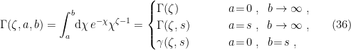
 and
and  are the upper and lower incomplete gamma functions, respectively, and
  with
with  . We then begin by defining a new variable
  , so that
 ,
,  (and broken the boldface convention, because I didn’t want to introduce even more letters). This is pretty close to the desired form already, but the complex exponent
  necessitates that we promote
  to a complex variable, and treat this as a contour integral in the complex plane.
 in the form
  with
with  , which has branch points at both
  and
and  , since there’s a non-trivial monodromy
  along a closed path that encircles either point in the complex plane. Since the integral converges as
  due to the exponential damping, let’s choose the branch cut to run from
  along the negative real axis, so that the following contour encloses no poles:
 , which vanishes since
  . Thus, taking
  along the positive complex axis, the integral (37) becomes
 . Comparing with the form of the gamma function (36), we identify
  and
and  , whence we find


 are similarly obtained from (27).
 , where the
  -vector
  , with Greek indices running over the full
  -dimensional spatial component. While I’m at it, I should also warn you that [1] uses the exceedingly unpalatable mostly-minus convention
  , whereas I’m going to use mostly-plus
  . The former seems to be preferred by particle physicists, because they share with small children a preference for timelike 4-vectors to have positive magnitude. But the latter is generally preferred by relativists and most workers in high-energy theory and quantum gravity, because 3-vectors have no minus signs (i.e., it’s consistent with the non-relativistic case, whereas mostly-plus yields a negative-definite metric), raising and lowering indices involves flipping only a single sign (arguably the most important for our purposes, since we’ll be Wick rotating between Lorentzian and Euclidean signature; mostly-plus would again lead to a negative-definite Euclidean metric), and the extension to general dimensions contains only a single
  in the determinant (as opposed to a factor of
  in mostly-minus).
 is the Minkowski metric (no curved space just yet). By applying the variational principle
  to the action

 . The general solution, upon imposing that
 ![\displaystyle \phi(x)=\int\!\frac{\mathrm{d}^dk}{2\omega(2\pi)^d}\left[a_k e^{i\mathbf{k}\mathbf{x}-i\omega t}+a_k^\dagger e^{-i\mathbf{k}\mathbf{x}+i\omega t}\right]~, \ \ \ \ \ (4)](https://s0.wp.com/latex.php?latex=%5Cdisplaystyle+%5Cphi%28x%29%3D%5Cint%5C%21%5Cfrac%7B%5Cmathrm%7Bd%7D%5Edk%7D%7B2%5Comega%282%5Cpi%29%5Ed%7D%5Cleft%5Ba_k+e%5E%7Bi%5Cmathbf%7Bk%7D%5Cmathbf%7Bx%7D-i%5Comega+t%7D%2Ba_k%5E%5Cdagger+e%5E%7B-i%5Cmathbf%7Bk%7D%5Cmathbf%7Bx%7D%2Bi%5Comega+t%7D%5Cright%5D%7E%2C+%5C+%5C+%5C+%5C+%5C+%284%29&bg=ffffff&fg=000000&s=0&c=20201002)
 is the annihilation operator that kills the vacuum state, i.e.,
  (so
(so  , which affects a number of later formulas, and can cause confusion when comparing different sources. The convention I’m using is physically well-motivated in that it makes the measure Lorentz invariant while encoding the on-shell condition
  . That is, the Lorentz invariant measure in the full
  . If we then impose the on-shell condition along with
  (in the form of the Heaviside function
  ), we have
 has a root at
  , then we may write
 . In the present case,
  , and
, and  (note that the Heaviside function will select the positive root). Thus
 and
and  . Mathematicians seem to prefer splitting this so that both
  and
and  get a factor of
  , but physicists favour simply attaching it all to the momentum, so that

 (or vice versa):

 and the like for failure to invest this time at the start).
 from the two-point correlator
  , including the familiar Feynman propagator. Following [1], we’ll denote the expectation values of the commutator and anticommutator as follows:
 ![\displaystyle \begin{aligned} iG(x,x')&=\langle\left[\phi(x),\phi(x')\right]\rangle=G^+\!(x,x')-G^-\!(x,x')~,\\ G^{(1)}(x,x')&=\langle\left\{\phi(x),\phi(x')\right\}\rangle=G^+\!(x,x')+G^-\!(x,x')~, \end{aligned} \ \ \ \ \ (12)](https://s0.wp.com/latex.php?latex=%5Cdisplaystyle+%5Cbegin%7Baligned%7D+iG%28x%2Cx%27%29%26%3D%5Clangle%5Cleft%5B%5Cphi%28x%29%2C%5Cphi%28x%27%29%5Cright%5D%5Crangle%3DG%5E%2B%5C%21%28x%2Cx%27%29-G%5E-%5C%21%28x%2Cx%27%29%7E%2C%5C%5C+G%5E%7B%281%29%7D%28x%2Cx%27%29%26%3D%5Clangle%5Cleft%5C%7B%5Cphi%28x%29%2C%5Cphi%28x%27%29%5Cright%5C%7D%5Crangle%3DG%5E%2B%5C%21%28x%2Cx%27%29%2BG%5E-%5C%21%28x%2Cx%27%29%7E%2C+%5Cend%7Baligned%7D+%5C+%5C+%5C+%5C+%5C+%2812%29&bg=ffffff&fg=000000&s=0&c=20201002)
 on the far right-hand sides are the so-called positive/negative frequency Wightman functions,

 acts only on
  ), it reduces to the Klein-Gordon equation above for the Wightman functions, from which the others follow.
 ) Feynman propagator, and

 , we have
![\displaystyle \begin{aligned} \square_x G_F=&-i\eta^{\mu0}\partial_\mu\left[\delta(t-t')G^+\!(x,x')-\delta(t'-t)G^-\!(x,x')\right]\\ &-i\eta^{\mu\nu}\partial_\mu\left[\Theta(t-t')\partial_\nu G^+\!(x,x')+\Theta(t'-t)\partial_\nu G^-\!(x,x')\right]~. \end{aligned} \ \ \ \ \ (18)](https://s0.wp.com/latex.php?latex=%5Cdisplaystyle+%5Cbegin%7Baligned%7D+%5Csquare_x+G_F%3D%26-i%5Ceta%5E%7B%5Cmu0%7D%5Cpartial_%5Cmu%5Cleft%5B%5Cdelta%28t-t%27%29G%5E%2B%5C%21%28x%2Cx%27%29-%5Cdelta%28t%27-t%29G%5E-%5C%21%28x%2Cx%27%29%5Cright%5D%5C%5C+%26-i%5Ceta%5E%7B%5Cmu%5Cnu%7D%5Cpartial_%5Cmu%5Cleft%5B%5CTheta%28t-t%27%29%5Cpartial_%5Cnu+G%5E%2B%5C%21%28x%2Cx%27%29%2B%5CTheta%28t%27-t%29%5Cpartial_%5Cnu+G%5E-%5C%21%28x%2Cx%27%29%5Cright%5D%7E.+%5Cend%7Baligned%7D+%5C+%5C+%5C+%5C+%5C+%2818%29&bg=ffffff&fg=000000&s=0&c=20201002)
![{{[\phi(t,\mathbf{x}),\phi(t,\mathbf{x}')]=0}}](https://s0.wp.com/latex.php?latex=%7B%7B%5B%5Cphi%28t%2C%5Cmathbf%7Bx%7D%29%2C%5Cphi%28t%2C%5Cmathbf%7Bx%7D%27%29%5D%3D0%7D%7D&bg=ffffff&fg=000000&s=0&c=20201002) means that in the first line,
means that in the first line,  . And since the delta function itself is even, this implies that the first two terms cancel, so we continue with just the second line:
![\displaystyle \begin{aligned} \square_x G_F=&-i\eta^{00}\left[\delta(t-t')\partial_0 G^+\!(x,x')-\delta(t'-t)\partial_0 G^-\!(x,x')\right]\\ &-i\eta^{\mu\nu}\left[\Theta(t-t')\partial_\mu\partial_\nu G^+\!(x,x')+\Theta(t'-t)\partial_\mu\partial_\nu G^-\!(x,x')\right]\\ =&\,\,i\delta(t-t')\left[\pi(x)\phi(x')-\phi(x')\pi(x)\right]\\ &-i\left[\Theta(t-t')\square_x G^+\!(x,x')+\Theta(t'-t)\square_x G^-\!(x,x')\right]~, \end{aligned} \ \ \ \ \ (19)](https://s0.wp.com/latex.php?latex=%5Cdisplaystyle+%5Cbegin%7Baligned%7D+%5Csquare_x+G_F%3D%26-i%5Ceta%5E%7B00%7D%5Cleft%5B%5Cdelta%28t-t%27%29%5Cpartial_0+G%5E%2B%5C%21%28x%2Cx%27%29-%5Cdelta%28t%27-t%29%5Cpartial_0+G%5E-%5C%21%28x%2Cx%27%29%5Cright%5D%5C%5C+%26-i%5Ceta%5E%7B%5Cmu%5Cnu%7D%5Cleft%5B%5CTheta%28t-t%27%29%5Cpartial_%5Cmu%5Cpartial_%5Cnu+G%5E%2B%5C%21%28x%2Cx%27%29%2B%5CTheta%28t%27-t%29%5Cpartial_%5Cmu%5Cpartial_%5Cnu+G%5E-%5C%21%28x%2Cx%27%29%5Cright%5D%5C%5C+%3D%26%5C%2C%5C%2Ci%5Cdelta%28t-t%27%29%5Cleft%5B%5Cpi%28x%29%5Cphi%28x%27%29-%5Cphi%28x%27%29%5Cpi%28x%29%5Cright%5D%5C%5C+%26-i%5Cleft%5B%5CTheta%28t-t%27%29%5Csquare_x+G%5E%2B%5C%21%28x%2Cx%27%29%2B%5CTheta%28t%27-t%29%5Csquare_x+G%5E-%5C%21%28x%2Cx%27%29%5Cright%5D%7E%2C+%5Cend%7Baligned%7D+%5C+%5C+%5C+%5C+%5C+%2819%29&bg=ffffff&fg=000000&s=0&c=20201002)
 . Then by (14), the second line will vanish for all values of
  when we add in the
  term of the wave operator, and the first line is just (minus) the equal-time commutator
 ![{[\phi(t,\mathbf{x}),\pi(t,\mathbf{x}')]=i\delta^d(\mathbf{x}-\mathbf{x}')}](https://s0.wp.com/latex.php?latex=%7B%5B%5Cphi%28t%2C%5Cmathbf%7Bx%7D%29%2C%5Cpi%28t%2C%5Cmathbf%7Bx%7D%27%29%5D%3Di%5Cdelta%5Ed%28%5Cmathbf%7Bx%7D-%5Cmathbf%7Bx%7D%27%29%7D&bg=ffffff&fg=000000&s=0&c=20201002) . Hence
. Hence
 ; similarly for
  and
and  .
. “propagators” is that, unlike the kernels
  , they represent the transition amplitude for a particle (virtual or otherwise) propagating from
  , subject to appropriate boundary conditions. To see this, consider the integral representation
 . Due to the poles at
  , we need to choose a suitable contour for the integral to be well-defined (analytically continuing to
  ). The particular choice of contour determines which of the kernels
 , we may absorb the sign into the integration variable, and identify
 :
:
 prescription, i.e., which of the poles we want to enclose with the choice of contour. Consider first the retarded propagator
  (where
  ). Conversely, when
  , we must close the contour in the negative half-plane so that
  , and the integral converges. Thus we should introduce factors of
  , and then take
  :
: ![\displaystyle \begin{aligned} G_R(x,x')&=\int\frac{\mathrm{d}^dk}{(2\pi)^D}e^{i\mathbf{k}(\mathbf{x}-\mathbf{x}')}\oint\mathrm{d} k_0\frac{e^{-ik_0(x_0-x'_0)}}{-2k_0}\left(\frac{1}{k_0-\sqrt{\mathbf{k}^2+m^2}+i\epsilon}+\frac{1}{k_0+\sqrt{\mathbf{k}^2+m^2}+i\epsilon}\right)\\ &=\Theta(x_0-x'_0)\int\frac{\mathrm{d}^dk}{(2\pi)^D}e^{i\mathbf{k}(\mathbf{x}-\mathbf{x}')}(2\pi i)\left(\frac{e^{-i\omega(x_0-x'_0)}}{-2\omega}+\frac{e^{i\omega(x_0-x'_0)}}{2\omega}\right)\\ &=-i\Theta(x_0-x'_0)\int\frac{\mathrm{d}^dk}{2\omega(2\pi)^d}e^{i\mathbf{k}(\mathbf{x}-\mathbf{x}')}\left( e^{-i\omega(x_0-x'_0)}-e^{i\omega(x_0-x'_0)}\right)\\ &=-i\Theta(x_0-x'_0)\int\frac{\mathrm{d}^dk}{2\omega(2\pi)^d}\left[e^{ik(x-x')}-e^{-ik(x-x')}\right]\\ &=i\Theta(x_0-x'_0)\langle\left[\phi(x),\phi(x')\right]\rangle =-\Theta(t-t')G(x,x')~, \end{aligned} \ \ \ \ \ (24)](https://s0.wp.com/latex.php?latex=%5Cdisplaystyle+%5Cbegin%7Baligned%7D+G_R%28x%2Cx%27%29%26%3D%5Cint%5Cfrac%7B%5Cmathrm%7Bd%7D%5Edk%7D%7B%282%5Cpi%29%5ED%7De%5E%7Bi%5Cmathbf%7Bk%7D%28%5Cmathbf%7Bx%7D-%5Cmathbf%7Bx%7D%27%29%7D%5Coint%5Cmathrm%7Bd%7D+k_0%5Cfrac%7Be%5E%7B-ik_0%28x_0-x%27_0%29%7D%7D%7B-2k_0%7D%5Cleft%28%5Cfrac%7B1%7D%7Bk_0-%5Csqrt%7B%5Cmathbf%7Bk%7D%5E2%2Bm%5E2%7D%2Bi%5Cepsilon%7D%2B%5Cfrac%7B1%7D%7Bk_0%2B%5Csqrt%7B%5Cmathbf%7Bk%7D%5E2%2Bm%5E2%7D%2Bi%5Cepsilon%7D%5Cright%29%5C%5C+%26%3D%5CTheta%28x_0-x%27_0%29%5Cint%5Cfrac%7B%5Cmathrm%7Bd%7D%5Edk%7D%7B%282%5Cpi%29%5ED%7De%5E%7Bi%5Cmathbf%7Bk%7D%28%5Cmathbf%7Bx%7D-%5Cmathbf%7Bx%7D%27%29%7D%282%5Cpi+i%29%5Cleft%28%5Cfrac%7Be%5E%7B-i%5Comega%28x_0-x%27_0%29%7D%7D%7B-2%5Comega%7D%2B%5Cfrac%7Be%5E%7Bi%5Comega%28x_0-x%27_0%29%7D%7D%7B2%5Comega%7D%5Cright%29%5C%5C+%26%3D-i%5CTheta%28x_0-x%27_0%29%5Cint%5Cfrac%7B%5Cmathrm%7Bd%7D%5Edk%7D%7B2%5Comega%282%5Cpi%29%5Ed%7De%5E%7Bi%5Cmathbf%7Bk%7D%28%5Cmathbf%7Bx%7D-%5Cmathbf%7Bx%7D%27%29%7D%5Cleft%28+e%5E%7B-i%5Comega%28x_0-x%27_0%29%7D-e%5E%7Bi%5Comega%28x_0-x%27_0%29%7D%5Cright%29%5C%5C+%26%3D-i%5CTheta%28x_0-x%27_0%29%5Cint%5Cfrac%7B%5Cmathrm%7Bd%7D%5Edk%7D%7B2%5Comega%282%5Cpi%29%5Ed%7D%5Cleft%5Be%5E%7Bik%28x-x%27%29%7D-e%5E%7B-ik%28x-x%27%29%7D%5Cright%5D%5C%5C+%26%3Di%5CTheta%28x_0-x%27_0%29%5Clangle%5Cleft%5B%5Cphi%28x%29%2C%5Cphi%28x%27%29%5Cright%5D%5Crangle+%3D-%5CTheta%28t-t%27%29G%28x%2Cx%27%29%7E%2C+%5Cend%7Baligned%7D+%5C+%5C+%5C+%5C+%5C+%2824%29&bg=ffffff&fg=000000&s=0&c=20201002)
![{[a_k,a_k'^\dagger]=2\omega(2\pi)^d\delta^d(\mathbf{k}-\mathbf{k}')}](https://s0.wp.com/latex.php?latex=%7B%5Ba_k%2Ca_k%27%5E%5Cdagger%5D%3D2%5Comega%282%5Cpi%29%5Ed%5Cdelta%5Ed%28%5Cmathbf%7Bk%7D-%5Cmathbf%7Bk%7D%27%29%7D&bg=ffffff&fg=000000&s=0&c=20201002) . Note that to yield the correct signs, we’ve chosen the contour to run counter-clockwise (note the factor of
. Note that to yield the correct signs, we’ve chosen the contour to run counter-clockwise (note the factor of  ), which means that it runs from
  to
to  along the real axis. The prescription for the advanced propagator is precisely similar, except we deform both poles in the positive complex direction (so that the integral vanishes when we close the contour below, as required for
  ), and the non-vanishing contribution comes from closing the contour in the positive half-plane, encircling both poles clockwise rather than counter-clockwise (so that the integral again runs from
  are superpositions of both positive (
 ) energy modes, which is necessary in order for them to vanish outside their prescribed lightcones (past and future, respectively). In contrast, the Heaviside functions in the Feynman propagator are tantamount to imposing boundary conditions such that it picks up only positive or negative frequencies, depending on the sign of
  , we close the contour in the lower-half plane for convergence (
 ), and enclose
  counter-clockwise (in the present conventions, we’re again going from
  when
when  . Hence the corresponding
 ![\displaystyle \begin{aligned} iG_F(x,x')&=i\int\frac{\mathrm{d}^dk}{(2\pi)^D}e^{i\mathbf{k}(\mathbf{x}-\mathbf{x}')}\oint\mathrm{d} k_0\frac{e^{-ik_0(x_0-x'_0)}}{-2k_0}\left(\frac{1}{k_0-\sqrt{\mathbf{k}^2+m^2}-i\epsilon}+\frac{1}{k_0+\sqrt{\mathbf{k}^2+m^2}+i\epsilon}\right)\\ &=i\int\frac{\mathrm{d}^dk}{(2\pi)^D}e^{i\mathbf{k}(\mathbf{x}-\mathbf{x}')}\left[(2\pi i)\Theta(x_0-x_0')\frac{e^{-i\omega(x_0-x'_0)}}{-2\omega}+(-2\pi i)\Theta(x_0'-x_0)\frac{e^{i\omega(x_0-x'_0)}}{2\omega}\right]\\ &=\int\frac{\mathrm{d}^dk}{2\omega(2\pi)^d}\left[\Theta(x_0-x_0')e^{ik(x-x')}+\Theta(x_0'-x_0)e^{-ik(x-x')}\right]\\ &=\Theta(t-t')G^+(x,x')+\Theta(t'-t)G^-(x,x')~, \end{aligned} \ \ \ \ \ (25)](https://s0.wp.com/latex.php?latex=%5Cdisplaystyle+%5Cbegin%7Baligned%7D+iG_F%28x%2Cx%27%29%26%3Di%5Cint%5Cfrac%7B%5Cmathrm%7Bd%7D%5Edk%7D%7B%282%5Cpi%29%5ED%7De%5E%7Bi%5Cmathbf%7Bk%7D%28%5Cmathbf%7Bx%7D-%5Cmathbf%7Bx%7D%27%29%7D%5Coint%5Cmathrm%7Bd%7D+k_0%5Cfrac%7Be%5E%7B-ik_0%28x_0-x%27_0%29%7D%7D%7B-2k_0%7D%5Cleft%28%5Cfrac%7B1%7D%7Bk_0-%5Csqrt%7B%5Cmathbf%7Bk%7D%5E2%2Bm%5E2%7D-i%5Cepsilon%7D%2B%5Cfrac%7B1%7D%7Bk_0%2B%5Csqrt%7B%5Cmathbf%7Bk%7D%5E2%2Bm%5E2%7D%2Bi%5Cepsilon%7D%5Cright%29%5C%5C+%26%3Di%5Cint%5Cfrac%7B%5Cmathrm%7Bd%7D%5Edk%7D%7B%282%5Cpi%29%5ED%7De%5E%7Bi%5Cmathbf%7Bk%7D%28%5Cmathbf%7Bx%7D-%5Cmathbf%7Bx%7D%27%29%7D%5Cleft%5B%282%5Cpi+i%29%5CTheta%28x_0-x_0%27%29%5Cfrac%7Be%5E%7B-i%5Comega%28x_0-x%27_0%29%7D%7D%7B-2%5Comega%7D%2B%28-2%5Cpi+i%29%5CTheta%28x_0%27-x_0%29%5Cfrac%7Be%5E%7Bi%5Comega%28x_0-x%27_0%29%7D%7D%7B2%5Comega%7D%5Cright%5D%5C%5C+%26%3D%5Cint%5Cfrac%7B%5Cmathrm%7Bd%7D%5Edk%7D%7B2%5Comega%282%5Cpi%29%5Ed%7D%5Cleft%5B%5CTheta%28x_0-x_0%27%29e%5E%7Bik%28x-x%27%29%7D%2B%5CTheta%28x_0%27-x_0%29e%5E%7B-ik%28x-x%27%29%7D%5Cright%5D%5C%5C+%26%3D%5CTheta%28t-t%27%29G%5E%2B%28x%2Cx%27%29%2B%5CTheta%28t%27-t%29G%5E-%28x%2Cx%27%29%7E%2C+%5Cend%7Baligned%7D+%5C+%5C+%5C+%5C+%5C+%2825%29&bg=ffffff&fg=000000&s=0&c=20201002)
 , we have a negative-energy particle (i.e., an antiparticle) propagating backwards.
 , is in any of the states
  with (classical) probability
 with respect to (26) are then ensemble averages at fixed temperature
  :
:
 — will fluctuate as quanta are created or destroyed. Strictly speaking I should also include the chemical potential, since the number operator
  also fluctuates, but it doesn’t play any important role in what follows. (The distinction is worth keeping in mind when discussing black hole thermodynamics, where one should use the microcanonical ensemble instead, because the negative specific heat makes the canonical ensemble unstable).
 , are then obtained by replacing the vacuum expectation value with the expectation value in the thermal state, (28); for example, the Wightman functions become
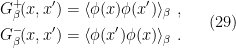

 :
:![\displaystyle \begin{aligned} G_\beta^+&=\frac{1}{Z}\mathrm{tr}\left[e^{-\beta H}\phi(t,\mathbf{x})\phi(t,\mathbf{x}')\right] =\frac{1}{Z}\mathrm{tr}\left[e^{-\beta H}\phi(t,\mathbf{x})e^{\beta H}e^{-\beta H}\phi(t,\mathbf{x}')\right]\\ &=\frac{1}{Z}\mathrm{tr}\left[\phi(t+i\beta,\mathbf{x})e^{-\beta H}\phi(t,\mathbf{x}')\right] =\frac{1}{Z}\mathrm{tr}\left[e^{-\beta H}\phi(t',\mathbf{x}')\phi(t+i\beta,\mathbf{x})\right]~, \end{aligned} \ \ \ \ \ (31)](https://s0.wp.com/latex.php?latex=%5Cdisplaystyle+%5Cbegin%7Baligned%7D+G_%5Cbeta%5E%2B%26%3D%5Cfrac%7B1%7D%7BZ%7D%5Cmathrm%7Btr%7D%5Cleft%5Be%5E%7B-%5Cbeta+H%7D%5Cphi%28t%2C%5Cmathbf%7Bx%7D%29%5Cphi%28t%2C%5Cmathbf%7Bx%7D%27%29%5Cright%5D+%3D%5Cfrac%7B1%7D%7BZ%7D%5Cmathrm%7Btr%7D%5Cleft%5Be%5E%7B-%5Cbeta+H%7D%5Cphi%28t%2C%5Cmathbf%7Bx%7D%29e%5E%7B%5Cbeta+H%7De%5E%7B-%5Cbeta+H%7D%5Cphi%28t%2C%5Cmathbf%7Bx%7D%27%29%5Cright%5D%5C%5C+%26%3D%5Cfrac%7B1%7D%7BZ%7D%5Cmathrm%7Btr%7D%5Cleft%5B%5Cphi%28t%2Bi%5Cbeta%2C%5Cmathbf%7Bx%7D%29e%5E%7B-%5Cbeta+H%7D%5Cphi%28t%2C%5Cmathbf%7Bx%7D%27%29%5Cright%5D+%3D%5Cfrac%7B1%7D%7BZ%7D%5Cmathrm%7Btr%7D%5Cleft%5Be%5E%7B-%5Cbeta+H%7D%5Cphi%28t%27%2C%5Cmathbf%7Bx%7D%27%29%5Cphi%28t%2Bi%5Cbeta%2C%5Cmathbf%7Bx%7D%29%5Cright%5D%7E%2C+%5Cend%7Baligned%7D+%5C+%5C+%5C+%5C+%5C+%2831%29&bg=ffffff&fg=000000&s=0&c=20201002)
 . Thus we arrive at the KMS condition

 .
. by an amount given by the (inverse) temperature
  , the finite-temperature field theory lives on
  , where
  (observe that as
  , we recover the zero temperature Euclidean theory on
 is the Schwarzschild radius, and
  is the metric on the
  sphere, which we’ll ignore since it just comes along for the ride. Recall from
 is the radial direction, and — since these are polar coordinates —
  takes on the role of the angular coordinate, which must be periodic to avoid a conical singularity; that is, for any integer
 .
. of neuron
  in layer
  is given by
 is some non-linear activation function of the neurons in the previous layer, and
  is an
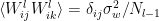
is an  matrix of weights. The qualifier “random” refers to the fact that the weights and biases are i.i.d. according to the normal distributions
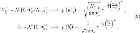
 has been introduced to ensure that the contribution from the previous layer remains
  regardless of layer width.
 as fixed, this is a linear combination of independent, normally-distributed variables, so we expect it to be Gaussian as well. Indeed, we can derive this rather easily by considering the characteristic function, which is a somewhat more fundamental way of characterizing probability distributions than the moment and cumulant generating functions we’ve discussed
  , the characteristic function is defined as
 exists. Hence for a Gaussian random variable
  , we have

 are independent random variables and
  are some constants. In the present case, we may view each
  as a constant modifying the random variable
 ![\displaystyle \begin{aligned} \phi_{z_i^l}(t)&=\phi_{b_i^l}(t)\prod_j\phi_{W_{ij}^l}(y_j^{l-1}t) =e^{-\frac{1}{2}\sigma_b^2t^2}\prod_je^{-\frac{1}{2N_{l-1}}\sigma_w^2(y_j^{l-1})^2}\\ &=\exp\left[-\frac{1}{2}\left(\sigma_w^2\frac{1}{N_{l-1}}\sum_j(y_j^{l-1})^2+\sigma_b^2\right) t^2\right]~. \end{aligned} \ \ \ \ \ (6)](https://s0.wp.com/latex.php?latex=%5Cdisplaystyle+%5Cbegin%7Baligned%7D+%5Cphi_%7Bz_i%5El%7D%28t%29%26%3D%5Cphi_%7Bb_i%5El%7D%28t%29%5Cprod_j%5Cphi_%7BW_%7Bij%7D%5El%7D%28y_j%5E%7Bl-1%7Dt%29+%3De%5E%7B-%5Cfrac%7B1%7D%7B2%7D%5Csigma_b%5E2t%5E2%7D%5Cprod_je%5E%7B-%5Cfrac%7B1%7D%7B2N_%7Bl-1%7D%7D%5Csigma_w%5E2%28y_j%5E%7Bl-1%7D%29%5E2%7D%5C%5C+%26%3D%5Cexp%5Cleft%5B-%5Cfrac%7B1%7D%7B2%7D%5Cleft%28%5Csigma_w%5E2%5Cfrac%7B1%7D%7BN_%7Bl-1%7D%7D%5Csum_j%28y_j%5E%7Bl-1%7D%29%5E2%2B%5Csigma_b%5E2%5Cright%29+t%5E2%5Cright%5D%7E.+%5Cend%7Baligned%7D+%5C+%5C+%5C+%5C+%5C+%286%29&bg=ffffff&fg=000000&s=0&c=20201002)

 limit
limit  becomes the variance of the distribution of inputs across the entire layer. The
  is cumbersome), we’ll introduce the notation
  to denote the variance of the pre-activations in layer
 to denote the standard normal Gaussian measure, and we’ve defined
  so that
  . That is, we can’t just write
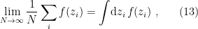
 . Specifically, it assumes that we’re integrating over the real line, whereas we know that
  in fact lie along a Gaussian. Thus we need a Lebesgue integral (rather than the more familiar Riemann integral) with an appropriate measure—in this case,
  . (We could alternatively have written
  , but it’s cleaner to simply rescale things). Substituting this back into (7), we thus obtain a recursion relation for the variance:
 to track particular inputs through the network, so that
  is the value of the
  neuron in layer
  ,
,  is its value in response to data
  , etc., where the data is fed into the network by setting
  (here boldface letters denote the entire layer, treated as a vector in
  ). We then consider the two-point correlator between these inputs at a single neuron:
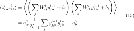
 , and that the weights and biases are independent with
  . Note that since
  , this also happens to be the covariance
  , which we shall denote
  in accordance with the notation from [1] introduced above.
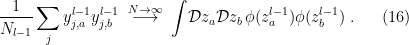
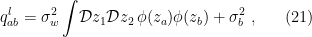
 and
and  , since that would preclude any correlation in the original inputs
  . Rather, any non-zero correlation in the data will propagate through the network, so the appropriate measure is the bivariate normal distribution,
![\displaystyle \mathcal{D} z_a\mathcal{D} z_b =\frac{\mathrm{d} z_a\mathrm{d} z_b}{2\pi\sqrt{q_a^{l-1}q_b^{l-1}(1-\rho^2)}}\, \exp\!\left[-\frac{1}{2(1-\rho^2)}\left(\frac{z_a^2}{q_a^{l-1}}+\frac{z_b^2}{q_b^{l-1}}-\frac{2\rho\,z_az_b}{\sqrt{q_a^{l-1}q_b^{l-1}}}\right)\right]~, \ \ \ \ \ (17)](https://s0.wp.com/latex.php?latex=%5Cdisplaystyle+%5Cmathcal%7BD%7D+z_a%5Cmathcal%7BD%7D+z_b+%3D%5Cfrac%7B%5Cmathrm%7Bd%7D+z_a%5Cmathrm%7Bd%7D+z_b%7D%7B2%5Cpi%5Csqrt%7Bq_a%5E%7Bl-1%7Dq_b%5E%7Bl-1%7D%281-%5Crho%5E2%29%7D%7D%5C%2C+%5Cexp%5C%21%5Cleft%5B-%5Cfrac%7B1%7D%7B2%281-%5Crho%5E2%29%7D%5Cleft%28%5Cfrac%7Bz_a%5E2%7D%7Bq_a%5E%7Bl-1%7D%7D%2B%5Cfrac%7Bz_b%5E2%7D%7Bq_b%5E%7Bl-1%7D%7D-%5Cfrac%7B2%5Crho%5C%2Cz_az_b%7D%7B%5Csqrt%7Bq_a%5E%7Bl-1%7Dq_b%5E%7Bl-1%7D%7D%7D%5Cright%29%5Cright%5D%7E%2C+%5C+%5C+%5C+%5C+%5C+%2817%29&bg=ffffff&fg=000000&s=0&c=20201002)

 by
by  . If the inputs are uncorrelated (i.e.,
  ), then
  , and the measure reduces to a product of independent Gaussian variables, as expected. (I say “as expected” because the individual inputs
  is only sensitive to linear relationships between random variables
  ; if these are related non-linearly, then it’s possible for them to be dependent (
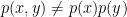 ) despite being uncorrelated (
 ). See Wikipedia for a
  such that

 given by (19). Note that since
  ) follows from their uncorrelatedness,
  ; the latter is easily shown by direct computation, and recalling that
  .
. ,
,  , which one can determine graphically (i.e., numerically) for a given choice of non-linear activation
  . For example, the case
  is plotted in fig. 1 of [1] (shown below), demonstrating that the fixed point condition
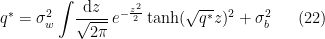
 . Therefore, when the parameters of the network (i.e., the distributions (2)) are tuned appropriately, the variance remains constant as signals propagate through the layers. This is useful, because it means that non-zero biases at each layer prevent signals from decaying to zero. Furthermore, provided the non-linearity
  , the dynamics ensures convergence to
  for all initial values. To visualize this, consider the following figure, which I took from [1] (
 is their notation for the recursion relation (14)). In the left plot, I’ve added the red arrows illustrating the convergence to the fixed point for
  . For the particular starting point I chose, it takes about 3 iterations to converge, which is consistent with the plot on the right.
 ,
,  . Hence by dividing (21) by
 ![\displaystyle \rho^l=\frac{\sigma_w^2}{q^*}\int\!\mathcal{D} z_1\mathcal{D} z_2\, \phi\left(\sqrt{q^*}z_1\right) \phi\left(\sqrt{q^*}\left[\rho^{l-1}z_1+\sqrt{1-(\rho^{l-1})^2}z_2\right]\right) +\frac{\sigma_b^2}{q^*}~. \ \ \ \ \ (23)](https://s0.wp.com/latex.php?latex=%5Cdisplaystyle+%5Crho%5El%3D%5Cfrac%7B%5Csigma_w%5E2%7D%7Bq%5E%2A%7D%5Cint%5C%21%5Cmathcal%7BD%7D+z_1%5Cmathcal%7BD%7D+z_2%5C%2C+%5Cphi%5Cleft%28%5Csqrt%7Bq%5E%2A%7Dz_1%5Cright%29+%5Cphi%5Cleft%28%5Csqrt%7Bq%5E%2A%7D%5Cleft%5B%5Crho%5E%7Bl-1%7Dz_1%2B%5Csqrt%7B1-%28%5Crho%5E%7Bl-1%7D%29%5E2%7Dz_2%5Cright%5D%5Cright%29+%2B%5Cfrac%7B%5Csigma_b%5E2%7D%7Bq%5E%2A%7D%7E.+%5C+%5C+%5C+%5C+%5C+%2823%29&bg=ffffff&fg=000000&s=0&c=20201002)
 :
:
 , and we have identified the single-neuron variance
  , cf. (14), which is
  .
. :
: 
 (the second equality is not obvious; see the derivation at the end of this post if you’re curious). The reason is that for monotonic functions
  implies that the curve (23) must approach the unity line from above (i.e., it’s concave, or has a constant slope with a vertical offset at
  set by the biases), and hence in this case
  is driven towards the fixed point
  , the curve must be approaching this point from below (i.e., it’s convex), and hence in this case
  . (It may help to sketch a few examples, like I superimposed on the left figure above, to convince yourself that this slope/convergence argument works).
 . At exactly
  , the system lies at a critical point, and should therefore be characterized some divergence(s) (recall that, in the limit
  , a phase transition is defined by the discontinuous change of some quantity; one often hears of an “
 order phase transition” if the discontinuity lies in the
  . To determine the fall-off behaviour, we expand near the critical point, and examine the difference
  as
as  (where recall
  . The limit simply ensures that
  exist; as shown above, we don’t have to wait that long in practice). This is done explicitly in [2], so I won’t work through all the details here; the result is that upon expanding
  , one finds the recurrence relation
 . This implies that, at least asymptotically,
  , which one can verify by substituting this into (26) and identifying
 ![\displaystyle \xi^{-1}=-\ln\left[\sigma_w^2\int\!\mathcal{D} z_1\mathcal{D} z_2\,\phi'(z_a)\phi'(z_b)\right]~. \ \ \ \ \ (27)](https://s0.wp.com/latex.php?latex=%5Cdisplaystyle+%5Cxi%5E%7B-1%7D%3D-%5Cln%5Cleft%5B%5Csigma_w%5E2%5Cint%5C%21%5Cmathcal%7BD%7D+z_1%5Cmathcal%7BD%7D+z_2%5C%2C%5Cphi%27%28z_a%29%5Cphi%27%28z_b%29%5Cright%5D%7E.+%5C+%5C+%5C+%5C+%5C+%2827%29&bg=ffffff&fg=000000&s=0&c=20201002)
 is the correlation length that governs the propagation of information — i.e., the decay of the two-point correlator — through the network. And again, we know from our discussion in
  , observe that the argument of (27) reduces to (25), i.e.,
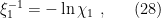
 , we expect that the basic conclusion about trainability above still holds even if the correlation length remains finite. And indeed, the main result of [2] is that at the critical point, not only can information about the inputs propagate all the way through the network, but information about the gradients can also propagate backwards (that is, exploding/vanishing gradients happen only in the ordered/chaotic phases, respectively, but are stable at the phase transition), and consequently these random networks are trainable provided
  .
.
 — denoted simply
  (cf.(19)), we have from (23)
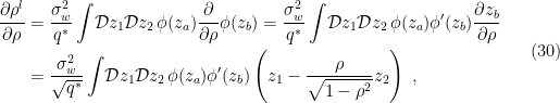
 . We therefore have the identities


 , whereupon the second term vanishes,

 , the ratio of depth to width (this works for most deep networks of practical interest, which typically have
  ). Finite-width corrections appear at
  , which physically correspond to effective interactions that arise upon marginalizing over hidden degrees of freedom; see my post on
  correction to the MFT (i.e., tree level) result, which is independent of network size, and therefore survives in the
  spins per direction):
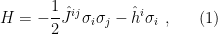
 , and for compactness I’m employing Einstein’s summation convention with
  and
and  . Since all directions are spacelike, there’s no difference between raised and lowered indices (e.g.,
  ), so I’ll denote the inverse matrix
  explicitly to avoid any possible confusion, i.e.,
  and
and  . In a 1d lattice, one would typically avoid boundary effects by joining the ends into an
  , but this issue won’t be relevant for our purposes, as we’ll be interested in the thermodynamic limit
  , the effect of all the other spins acts like an external magnetic field. That is, observe that we may write (1) as
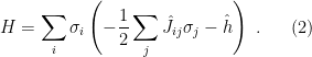
 by the average value,
  . We’ll give a more thorough Bayesian treatment of MFT below, but the idea here is that since no spin is special, the most likely value of
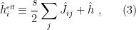
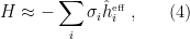
 . This is illustrated explicitly in John McGreevy’s entertaining
 ![\displaystyle \begin{aligned} \sigma_i\sigma_i&=\left[s+(\sigma_i-s)\right]\left[s+(\sigma_j-s)\right] =\left( s+\delta s_i\right)\left( s+\delta s_j\right)\\ &=s^2+s\left( \delta s_i+\delta s_j\right)+O(\delta s^2) =-s^2+s\left(\sigma_i+\sigma_j\right)+O(\delta s^2)~, \end{aligned} \ \ \ \ \ (5)](https://s0.wp.com/latex.php?latex=%5Cdisplaystyle+%5Cbegin%7Baligned%7D+%5Csigma_i%5Csigma_i%26%3D%5Cleft%5Bs%2B%28%5Csigma_i-s%29%5Cright%5D%5Cleft%5Bs%2B%28%5Csigma_j-s%29%5Cright%5D+%3D%5Cleft%28+s%2B%5Cdelta+s_i%5Cright%29%5Cleft%28+s%2B%5Cdelta+s_j%5Cright%29%5C%5C+%26%3Ds%5E2%2Bs%5Cleft%28+%5Cdelta+s_i%2B%5Cdelta+s_j%5Cright%29%2BO%28%5Cdelta+s%5E2%29+%3D-s%5E2%2Bs%5Cleft%28%5Csigma_i%2B%5Csigma_j%5Cright%29%2BO%28%5Cdelta+s%5E2%29%7E%2C+%5Cend%7Baligned%7D+%5C+%5C+%5C+%5C+%5C+%285%29&bg=ffffff&fg=000000&s=0&c=20201002)
 . We then substitute this into the hamiltonian (1); taking
  for simplicity, we obtain
 , this procedure yields the Boltzmann distribution
 ![\displaystyle p_i\equiv p(x_i)=\frac{1}{Z[\beta]}e^{-\beta E_i}~, \qquad\qquad\sum_ip_i=1~, \ \ \ \ \ (7)](https://s0.wp.com/latex.php?latex=%5Cdisplaystyle+p_i%5Cequiv+p%28x_i%29%3D%5Cfrac%7B1%7D%7BZ%5B%5Cbeta%5D%7De%5E%7B-%5Cbeta+E_i%7D%7E%2C+%5Cqquad%5Cqquad%5Csum_ip_i%3D1%7E%2C+%5C+%5C+%5C+%5C+%5C+%287%29&bg=ffffff&fg=000000&s=0&c=20201002)
 , and we identify the inverse temperature
![{Z[\beta]=e^{\beta\lambda}}](https://s0.wp.com/latex.php?latex=%7BZ%5B%5Cbeta%5D%3De%5E%7B%5Cbeta%5Clambda%7D%7D&bg=ffffff&fg=000000&s=0&c=20201002) where
where  is the Lagrange multiplier for the normalization constraint, cf. the max-ent procedure
  , provides an upper bound on the true (equilibrium) free energy
  :
:
 (henceforth I’ll refer to this simply as the free energy, without the “normalized” qualifier). This statement, sometimes referred to as the Bogolyubov inequality, can be
 ![\displaystyle \begin{aligned} Z_\textrm{\tiny{MF}}&=\sum_{\{\sigma\}}e^{-\beta H_\textrm{\tiny{MF}}} =\prod_{k=1}^N\sum_{\sigma_k=\pm1}\exp\left[-NdJs^2+\left(2dJs+h\right)\sum_i\sigma_i\right]\\ &=e^{-NdJs^2}\prod_{k=1}^N\exp\left[-\left(2dJs+h\right)+\left(2dJs+h\right)\right]\\ &=2^Ne^{-NdJs^2}\cosh^N\left(2dJs+h\right)~. \end{aligned} \ \ \ \ \ (10)](https://s0.wp.com/latex.php?latex=%5Cdisplaystyle+%5Cbegin%7Baligned%7D+Z_%5Ctextrm%7B%5Ctiny%7BMF%7D%7D%26%3D%5Csum_%7B%5C%7B%5Csigma%5C%7D%7De%5E%7B-%5Cbeta+H_%5Ctextrm%7B%5Ctiny%7BMF%7D%7D%7D+%3D%5Cprod_%7Bk%3D1%7D%5EN%5Csum_%7B%5Csigma_k%3D%5Cpm1%7D%5Cexp%5Cleft%5B-NdJs%5E2%2B%5Cleft%282dJs%2Bh%5Cright%29%5Csum_i%5Csigma_i%5Cright%5D%5C%5C+%26%3De%5E%7B-NdJs%5E2%7D%5Cprod_%7Bk%3D1%7D%5EN%5Cexp%5Cleft%5B-%5Cleft%282dJs%2Bh%5Cright%29%2B%5Cleft%282dJs%2Bh%5Cright%29%5Cright%5D%5C%5C+%26%3D2%5ENe%5E%7B-NdJs%5E2%7D%5Ccosh%5EN%5Cleft%282dJs%2Bh%5Cright%29%7E.+%5Cend%7Baligned%7D+%5C+%5C+%5C+%5C+%5C+%2810%29&bg=ffffff&fg=000000&s=0&c=20201002)
 neighbors with coupling strength
  and
and  ). The corresponding free energy is then
 term, since this doesn’t contribute to any of the observables for which
  :
: 
 , it looks as though
  , and therefore
 . Substituting in (3) for the homogeneous nearest-neighbor case at hand (that is, without the factor of
  , cf. (6)) then gives precisely (12).
 , the global minimum of
  is given by the intersection at positive
  in contrast, there’s a single minimum at
  for high temperatures, and two degenerate minima at
  at low temperatures (depending on whether
  crosses
  ; to see this, recall that for small
  , so a sufficiently small value of
 ,
,  , while for
  ,
,  ; we’ll have more to say about this failure below.
 will always be small (
 ) independent of
  (since
  ), so we can expand


 changes at the critical temperature
  , which determines whether the global minimum of
  (
( ) or
) or  (
( ). The physical interpretation is that below the critical temperature, it is energetically favourable for the spins to align, resulting in a non-zero magnetization (which is what the average spin
  is). Above the critical temperature however, thermal fluctuations disrupt this ordering, so the net magnetization is zero. For this reason, the magnetization
 ,
,  . The first step is to apply the Hubbard-Stratanovich transformation,
 ![\displaystyle e^{\frac{1}{2}K^{ij}s_is_j}=\left[\frac{\mathrm{det}K}{(2\pi)^N}\right]^{1/2}\!\int\!\mathrm{d}^N\phi\exp\left(-\frac{1}{2}K^{ij}\phi_i\phi_j+K^{ij}s_i\phi_j\right)~, \qquad\forall\,s_i\in\mathbb{R}~. \ \ \ \ \ (19)](https://s0.wp.com/latex.php?latex=%5Cdisplaystyle+e%5E%7B%5Cfrac%7B1%7D%7B2%7DK%5E%7Bij%7Ds_is_j%7D%3D%5Cleft%5B%5Cfrac%7B%5Cmathrm%7Bdet%7DK%7D%7B%282%5Cpi%29%5EN%7D%5Cright%5D%5E%7B1%2F2%7D%5C%21%5Cint%5C%21%5Cmathrm%7Bd%7D%5EN%5Cphi%5Cexp%5Cleft%28-%5Cfrac%7B1%7D%7B2%7DK%5E%7Bij%7D%5Cphi_i%5Cphi_j%2BK%5E%7Bij%7Ds_i%5Cphi_j%5Cright%29%7E%2C+%5Cqquad%5Cforall%5C%2Cs_i%5Cin%5Cmathbb%7BR%7D%7E.+%5C+%5C+%5C+%5C+%5C+%2819%29&bg=ffffff&fg=000000&s=0&c=20201002)
 ). Applying this transformation to the first term in the partition function, we have
 ![\displaystyle Z=\left[\frac{\mathrm{det}J}{(2\pi)^N}\right]^{1/2}\!\int\!\mathrm{d}^N\phi\sum_{\{\sigma\}}\exp\left[-\frac{1}{2}J^{ij}\phi_i\phi_j+\left( J^{ij}\phi_j+h^i\right)\sigma_i\right]~. \ \ \ \ \ (20)](https://s0.wp.com/latex.php?latex=%5Cdisplaystyle+Z%3D%5Cleft%5B%5Cfrac%7B%5Cmathrm%7Bdet%7DJ%7D%7B%282%5Cpi%29%5EN%7D%5Cright%5D%5E%7B1%2F2%7D%5C%21%5Cint%5C%21%5Cmathrm%7Bd%7D%5EN%5Cphi%5Csum_%7B%5C%7B%5Csigma%5C%7D%7D%5Cexp%5Cleft%5B-%5Cfrac%7B1%7D%7B2%7DJ%5E%7Bij%7D%5Cphi_i%5Cphi_j%2B%5Cleft%28+J%5E%7Bij%7D%5Cphi_j%2Bh%5Ei%5Cright%29%5Csigma_i%5Cright%5D%7E.+%5C+%5C+%5C+%5C+%5C+%2820%29&bg=ffffff&fg=000000&s=0&c=20201002)
 , leaving us with an expression entirely in terms of the new field variables
 ![\displaystyle \sum_{\sigma_i=\pm1}\exp\left[\left( J^{ij}\phi_j+h^i\right)\sigma_i\right]=2\cosh\left( J^{ij}\phi_j+h^i\right)~, \ \ \ \ \ (21)](https://s0.wp.com/latex.php?latex=%5Cdisplaystyle+%5Csum_%7B%5Csigma_i%3D%5Cpm1%7D%5Cexp%5Cleft%5B%5Cleft%28+J%5E%7Bij%7D%5Cphi_j%2Bh%5Ei%5Cright%29%5Csigma_i%5Cright%5D%3D2%5Ccosh%5Cleft%28+J%5E%7Bij%7D%5Cphi_j%2Bh%5Ei%5Cright%29%7E%2C+%5C+%5C+%5C+%5C+%5C+%2821%29&bg=ffffff&fg=000000&s=0&c=20201002)
![\displaystyle Z=\left[\left(\frac{2}{\pi}\right)^N\!\mathrm{det}J\right]^{1/2}\!\int\!\mathrm{d}^N\phi\exp\!\left[-\frac{1}{2}J^{ij}\phi_i\phi_j+\sum_i\ln\cosh\left( J^{ij}\phi_j+h^i\right)\right]~. \ \ \ \ \ (22)](https://s0.wp.com/latex.php?latex=%5Cdisplaystyle+Z%3D%5Cleft%5B%5Cleft%28%5Cfrac%7B2%7D%7B%5Cpi%7D%5Cright%29%5EN%5C%21%5Cmathrm%7Bdet%7DJ%5Cright%5D%5E%7B1%2F2%7D%5C%21%5Cint%5C%21%5Cmathrm%7Bd%7D%5EN%5Cphi%5Cexp%5C%21%5Cleft%5B-%5Cfrac%7B1%7D%7B2%7DJ%5E%7Bij%7D%5Cphi_i%5Cphi_j%2B%5Csum_i%5Cln%5Ccosh%5Cleft%28+J%5E%7Bij%7D%5Cphi_j%2Bh%5Ei%5Cright%29%5Cright%5D%7E.+%5C+%5C+%5C+%5C+%5C+%2822%29&bg=ffffff&fg=000000&s=0&c=20201002)
 can be thought of as the mean field
  at site
  by inverting this identification:
 , that
![\displaystyle Z=\left[\left(\frac{2}{\pi}\right)^N\!\mathrm{det}J^{-1}\right]^{1/2}\!e^{-\frac{1}{2}J^{-1}_{ij}h^ih^j}\!\int\!\mathrm{d}^N\!\mu\exp\!\left[-\frac{1}{2}J^{-1}_{ij}\mu^i\mu^j+J^{-1}_{ij}h^i\mu^j+\sum_i\ln\cosh\mu_i\right]~, \ \ \ \ \ (25)](https://s0.wp.com/latex.php?latex=%5Cdisplaystyle+Z%3D%5Cleft%5B%5Cleft%28%5Cfrac%7B2%7D%7B%5Cpi%7D%5Cright%29%5EN%5C%21%5Cmathrm%7Bdet%7DJ%5E%7B-1%7D%5Cright%5D%5E%7B1%2F2%7D%5C%21e%5E%7B-%5Cfrac%7B1%7D%7B2%7DJ%5E%7B-1%7D_%7Bij%7Dh%5Eih%5Ej%7D%5C%21%5Cint%5C%21%5Cmathrm%7Bd%7D%5EN%5C%21%5Cmu%5Cexp%5C%21%5Cleft%5B-%5Cfrac%7B1%7D%7B2%7DJ%5E%7B-1%7D_%7Bij%7D%5Cmu%5Ei%5Cmu%5Ej%2BJ%5E%7B-1%7D_%7Bij%7Dh%5Ei%5Cmu%5Ej%2B%5Csum_i%5Cln%5Ccosh%5Cmu_i%5Cright%5D%7E%2C+%5C+%5C+%5C+%5C+%5C+%2825%29&bg=ffffff&fg=000000&s=0&c=20201002)
 . We can then expand
![\displaystyle Z\approx\left[\left(\frac{2}{\pi}\right)^N\!\mathrm{det}J^{-1}\right]^{1/2}\!e^{-\frac{1}{2}J^{-1}_{ij}h^ih^j}\!\int\!\mathrm{d}^N\mu\exp\!\left[-\frac{1}{2}J^{-1}_{ij}\mu^i\mu^j +J^{-1}_{ij}h^i\mu^j +\sum_i\left(\frac{1}{2}\mu_i^2-\frac{1}{12}\mu_i^4\right)\right]~. \ \ \ \ \ (27)](https://s0.wp.com/latex.php?latex=%5Cdisplaystyle+Z%5Capprox%5Cleft%5B%5Cleft%28%5Cfrac%7B2%7D%7B%5Cpi%7D%5Cright%29%5EN%5C%21%5Cmathrm%7Bdet%7DJ%5E%7B-1%7D%5Cright%5D%5E%7B1%2F2%7D%5C%21e%5E%7B-%5Cfrac%7B1%7D%7B2%7DJ%5E%7B-1%7D_%7Bij%7Dh%5Eih%5Ej%7D%5C%21%5Cint%5C%21%5Cmathrm%7Bd%7D%5EN%5Cmu%5Cexp%5C%21%5Cleft%5B-%5Cfrac%7B1%7D%7B2%7DJ%5E%7B-1%7D_%7Bij%7D%5Cmu%5Ei%5Cmu%5Ej+%2BJ%5E%7B-1%7D_%7Bij%7Dh%5Ei%5Cmu%5Ej+%2B%5Csum_i%5Cleft%28%5Cfrac%7B1%7D%7B2%7D%5Cmu_i%5E2-%5Cfrac%7B1%7D%7B12%7D%5Cmu_i%5E4%5Cright%29%5Cright%5D%7E.+%5C+%5C+%5C+%5C+%5C+%2827%29&bg=ffffff&fg=000000&s=0&c=20201002)
 (i.e.,
  and
and  ), and obtain the path-integral measure
![\displaystyle \left[\left(\frac{2}{\pi}\right)^N\!\mathrm{det}J^{-1}\right]^{1/2}\!e^{-\frac{1}{2}J^{-1}_{ij}h^ih^j}\!\int\!\mathrm{d}^N\mu \;\longrightarrow\;\mathcal{N}\!\int\!\mathcal{D}\mu~. \ \ \ \ \ (28)](https://s0.wp.com/latex.php?latex=%5Cdisplaystyle+%5Cleft%5B%5Cleft%28%5Cfrac%7B2%7D%7B%5Cpi%7D%5Cright%29%5EN%5C%21%5Cmathrm%7Bdet%7DJ%5E%7B-1%7D%5Cright%5D%5E%7B1%2F2%7D%5C%21e%5E%7B-%5Cfrac%7B1%7D%7B2%7DJ%5E%7B-1%7D_%7Bij%7Dh%5Eih%5Ej%7D%5C%21%5Cint%5C%21%5Cmathrm%7Bd%7D%5EN%5Cmu+%5C%3B%5Clongrightarrow%5C%3B%5Cmathcal%7BN%7D%5C%21%5Cint%5C%21%5Cmathcal%7BD%7D%5Cmu%7E.+%5C+%5C+%5C+%5C+%5C+%2828%29&bg=ffffff&fg=000000&s=0&c=20201002)
![\displaystyle \begin{aligned} Z\approx\mathcal{N}\!\int\!\mathcal{D}\mu\exp\bigg\{\!&-\frac{1}{2}\int\!\mathrm{d}\mathbf{x}\mathrm{d}\mathbf{y}\,\mu(\mathbf{x})J^{-1}(\mathbf{x}-\mathbf{y})\big[\mu(\mathbf{y})-h\big]\\ &+\frac{1}{2}\int\!\mathrm{d}\mathbf{x}\left[\mu(\mathbf{x})^2-\frac{1}{6}\mu(\mathbf{x})^4\right]\bigg\}~, \end{aligned} \ \ \ \ \ (29)](https://s0.wp.com/latex.php?latex=%5Cdisplaystyle+%5Cbegin%7Baligned%7D+Z%5Capprox%5Cmathcal%7BN%7D%5C%21%5Cint%5C%21%5Cmathcal%7BD%7D%5Cmu%5Cexp%5Cbigg%5C%7B%5C%21%26-%5Cfrac%7B1%7D%7B2%7D%5Cint%5C%21%5Cmathrm%7Bd%7D%5Cmathbf%7Bx%7D%5Cmathrm%7Bd%7D%5Cmathbf%7By%7D%5C%2C%5Cmu%28%5Cmathbf%7Bx%7D%29J%5E%7B-1%7D%28%5Cmathbf%7Bx%7D-%5Cmathbf%7By%7D%29%5Cbig%5B%5Cmu%28%5Cmathbf%7By%7D%29-h%5Cbig%5D%5C%5C+%26%2B%5Cfrac%7B1%7D%7B2%7D%5Cint%5C%21%5Cmathrm%7Bd%7D%5Cmathbf%7Bx%7D%5Cleft%5B%5Cmu%28%5Cmathbf%7Bx%7D%29%5E2-%5Cfrac%7B1%7D%7B6%7D%5Cmu%28%5Cmathbf%7Bx%7D%29%5E4%5Cright%5D%5Cbigg%5C%7D%7E%2C+%5Cend%7Baligned%7D+%5C+%5C+%5C+%5C+%5C+%2829%29&bg=ffffff&fg=000000&s=0&c=20201002)
 , since the external magnetic field is the same for all lattice sites, cf. the definition of
  below (1).
 , except that it be a symmetric invertible matrix, with no self-interactions (
 and Taylor expand the field
  around
 as mediating interactions between fields at infinitesimally separated points in space, with increasingly non-local (i.e., higher-derivative) terms suppressed by powers of the separation. Upon substituting this expansion into (29), and working to second-order in this local expansion, one obtains a partition function of the form
 ![\displaystyle Z\approx\mathcal{N}\!\int\!\mathcal{D}\mu\,e^{-S[\mu]}~, \ \ \ \ \ (31)](https://s0.wp.com/latex.php?latex=%5Cdisplaystyle+Z%5Capprox%5Cmathcal%7BN%7D%5C%21%5Cint%5C%21%5Cmathcal%7BD%7D%5Cmu%5C%2Ce%5E%7B-S%5B%5Cmu%5D%7D%7E%2C+%5C+%5C+%5C+%5C+%5C+%2831%29&bg=ffffff&fg=000000&s=0&c=20201002)
![\displaystyle S[\mu]=\int\!\mathrm{d}^d\mathbf{x}\left[\frac{1}{2}\kappa(\nabla\mu)^2-h\mu+\frac{1}{2}\tilde r\mu^2+\frac{\tilde g}{4!}\mu^4\right]~, \ \ \ \ \ (32)](https://s0.wp.com/latex.php?latex=%5Cdisplaystyle+S%5B%5Cmu%5D%3D%5Cint%5C%21%5Cmathrm%7Bd%7D%5Ed%5Cmathbf%7Bx%7D%5Cleft%5B%5Cfrac%7B1%7D%7B2%7D%5Ckappa%28%5Cnabla%5Cmu%29%5E2-h%5Cmu%2B%5Cfrac%7B1%7D%7B2%7D%5Ctilde+r%5Cmu%5E2%2B%5Cfrac%7B%5Ctilde+g%7D%7B4%21%7D%5Cmu%5E4%5Cright%5D%7E%2C+%5C+%5C+%5C+%5C+%5C+%2832%29&bg=ffffff&fg=000000&s=0&c=20201002)
 ,
,  , and
, and  are some (analytic) functions of the physical parameters, and can be expressed in terms of the zero modes of the inverse coupling matrix. I’m not going to go through the details of that computation here, since a great exposition is already available in the answer to
  term).
 , and expanding the action to second order in the fluctuations
  , we have
 ![\displaystyle Z\approx\mathcal{N} e^{-S[\mu_0]}\int\!\mathcal{D}\mu\,e^{-\frac{1}{2}(\mu-\mu_0)^2S''[\mu_0]}~, \ \ \ \ \ (33)](https://s0.wp.com/latex.php?latex=%5Cdisplaystyle+Z%5Capprox%5Cmathcal%7BN%7D+e%5E%7B-S%5B%5Cmu_0%5D%7D%5Cint%5C%21%5Cmathcal%7BD%7D%5Cmu%5C%2Ce%5E%7B-%5Cfrac%7B1%7D%7B2%7D%28%5Cmu-%5Cmu_0%29%5E2S%27%27%5B%5Cmu_0%5D%7D%7E%2C+%5C+%5C+%5C+%5C+%5C+%2833%29&bg=ffffff&fg=000000&s=0&c=20201002)
 , and the linear term has vanished by definition, i.e.,
![\displaystyle Z\approx\mathcal{N} e^{-S[\mu_0]} \quad\mathrm{with}\quad S[\mu_0]=\int\!\mathrm{d}^d\mathbf{x}\left(\tilde r\mu_0^2+\frac{\tilde g}{8}\mu_0^4-\frac{3}{2}h\mu_0\right)~, \ \ \ \ \ (35)](https://s0.wp.com/latex.php?latex=%5Cdisplaystyle+Z%5Capprox%5Cmathcal%7BN%7D+e%5E%7B-S%5B%5Cmu_0%5D%7D+%5Cquad%5Cmathrm%7Bwith%7D%5Cquad+S%5B%5Cmu_0%5D%3D%5Cint%5C%21%5Cmathrm%7Bd%7D%5Ed%5Cmathbf%7Bx%7D%5Cleft%28%5Ctilde+r%5Cmu_0%5E2%2B%5Cfrac%7B%5Ctilde+g%7D%7B8%7D%5Cmu_0%5E4-%5Cfrac%7B3%7D%7B2%7Dh%5Cmu_0%5Cright%29%7E%2C+%5C+%5C+%5C+%5C+%5C+%2835%29&bg=ffffff&fg=000000&s=0&c=20201002)

 term. In the second equality, we have simply extracted the factor of
  (cf. the absorption of
  in (18), and the definition of
  ,
,  , and
, and  . For
. For ![{S''[\mu_0]}](https://s0.wp.com/latex.php?latex=%7BS%27%27%5B%5Cmu_0%5D%7D&bg=ffffff&fg=000000&s=0&c=20201002) , we have the operator
, we have the operator
 . Substituting this into (33) and doing the Gaussian integral, one finds that the contribution from this term is given by the sum of the eigenvalues of the operator
  . I’m not going to go through this in detail, since this post is getting long-winded, and
  , but the fluctuations diverge in
  and hence render its conclusions invalid. We’ll give a better explanation for this dimensional-dependent validity below.
 symmetry if
  , so the squared mass
  , a sextic coupling would have dimension
  , and so on. Recall that a coupling is relevant if its mass dimension
  (since the dimensionless coupling carries a factor of
  , e.g.,
  ), irrelevant if
  (since it runs like
  ), and marginal if
  . Thus we see that the quadratic term is always relevant, and that higher-order corrections are increasingly suppressed under RG in a dimension-dependent manner.
 term in the saddle point — is to compute the Gaussian path integral consisting of only the quadratic contribution, and treat the quartic and higher terms perturbatively. (As these originally arose from higher-order terms in the Taylor expansion, this is morally in line with simply taking
  in the MFT result
  ). Treating the action as a Gaussian integral also allows us to obtain a simple expression for the two-point correlator that captures the limiting behaviour in which we’re primarily interested. That is, tying all this back to the information theory / neural network connections alluded in the introduction, we’re ultimately interested in understanding the propagation of information near the critical point, so understanding how correlation functions behave in the leading-order / MFT / saddle point approximation — and how perturbative corrections from fluctuations might affect this — is of prime importance.
![\displaystyle S[\mu]=\int\!\mathrm{d}^d\mathbf{x}\left[\frac{1}{2}(\nabla\mu(\mathbf{x}))^2+\frac{m^2}{2}\mu(\mathbf{x})^2-h\mu(\mathbf{x})\right]~, \ \ \ \ \ (38)](https://s0.wp.com/latex.php?latex=%5Cdisplaystyle+S%5B%5Cmu%5D%3D%5Cint%5C%21%5Cmathrm%7Bd%7D%5Ed%5Cmathbf%7Bx%7D%5Cleft%5B%5Cfrac%7B1%7D%7B2%7D%28%5Cnabla%5Cmu%28%5Cmathbf%7Bx%7D%29%29%5E2%2B%5Cfrac%7Bm%5E2%7D%7B2%7D%5Cmu%28%5Cmathbf%7Bx%7D%29%5E2-h%5Cmu%28%5Cmathbf%7Bx%7D%29%5Cright%5D%7E%2C+%5C+%5C+%5C+%5C+%5C+%2838%29&bg=ffffff&fg=000000&s=0&c=20201002)
 and relabelled the quadratic coefficient
  . Evaluating partition functions of this type is a typical exercise in one’s first QFT course, since the action now resembles that of a free massive scalar field, where
  plays the role of the source (normally denoted
 merely serves as a mnemonic, and
  is the same field in momentum space. In the second equality, we’ve simply Fourier transformed back to real space by identifying the propagator
 . To see that this is indeed a correlation function,
 ,
,

 , and use the identity

 (not to be confused with the old name for the quadratic coefficient).
 and
and  , it is more illuminating to evaluate the integral via saddle point, rather than to preserve the exact form (which, as it turns out, can be expressed as a Bessel function). We thus exponentiate the
  factor to write

 is given by

 near the critical point, we see that the correlation length diverges as
 .
. 
 is the mean field from above, and in the last step we have used the scaling behaviours of
  and
and  (the latter can be obtained by minimizing the quartic result for
  dimensions. (The case
  actually requires a more careful RG treatment due to the logarithmic divergence; see Tong’s
  (here “
 ” means “proportional to”; we’ll fix the coefficient later).
 . Indeed, one of the most remarkable aspects of black holes is that the entropy scales with the area instead of the volume. Insofar as black holes represent the densest possible configuration of energy — and hence of information — this implies a drastic reduction in the (maximum) number of degrees of freedom in the universe, as I’ll discuss in more detail below. However, area laws for entanglement entropy are actually quite common; see for example [3] for a review. And while the ultimate source of black hole entropy (that is, the microscopic degrees of freedom it’s counting) is an ongoing topic of current research, the entanglement between the interior and exterior certainly plays an important role. But that’s a QFT calculation, whereas everything I’ve said so far is purely classical. Is there any way to see that the entropy must scale with
  instead of
 is the Schwarzschild radius and
  . For
. For  , the metric is static: the spatial components look the same for any value of
  , and hence
  . This makes the
  component positive and the
  component negative, so that space and time switch roles in the black hole interior. Consequently, the “spatial” components are no longer static inside the black hole, since they will continue to evolve with
  on that slice. But when space is curved, there are many different constant-
 is the determinant of the (induced) metric on
  , so we have
 , and the integral vanishes. Thus the Schwarzschild metric would lead one to conclude that the “volume” of the black hole is zero! (Technically the integral is ill-defined at
  and taking the limit
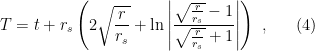

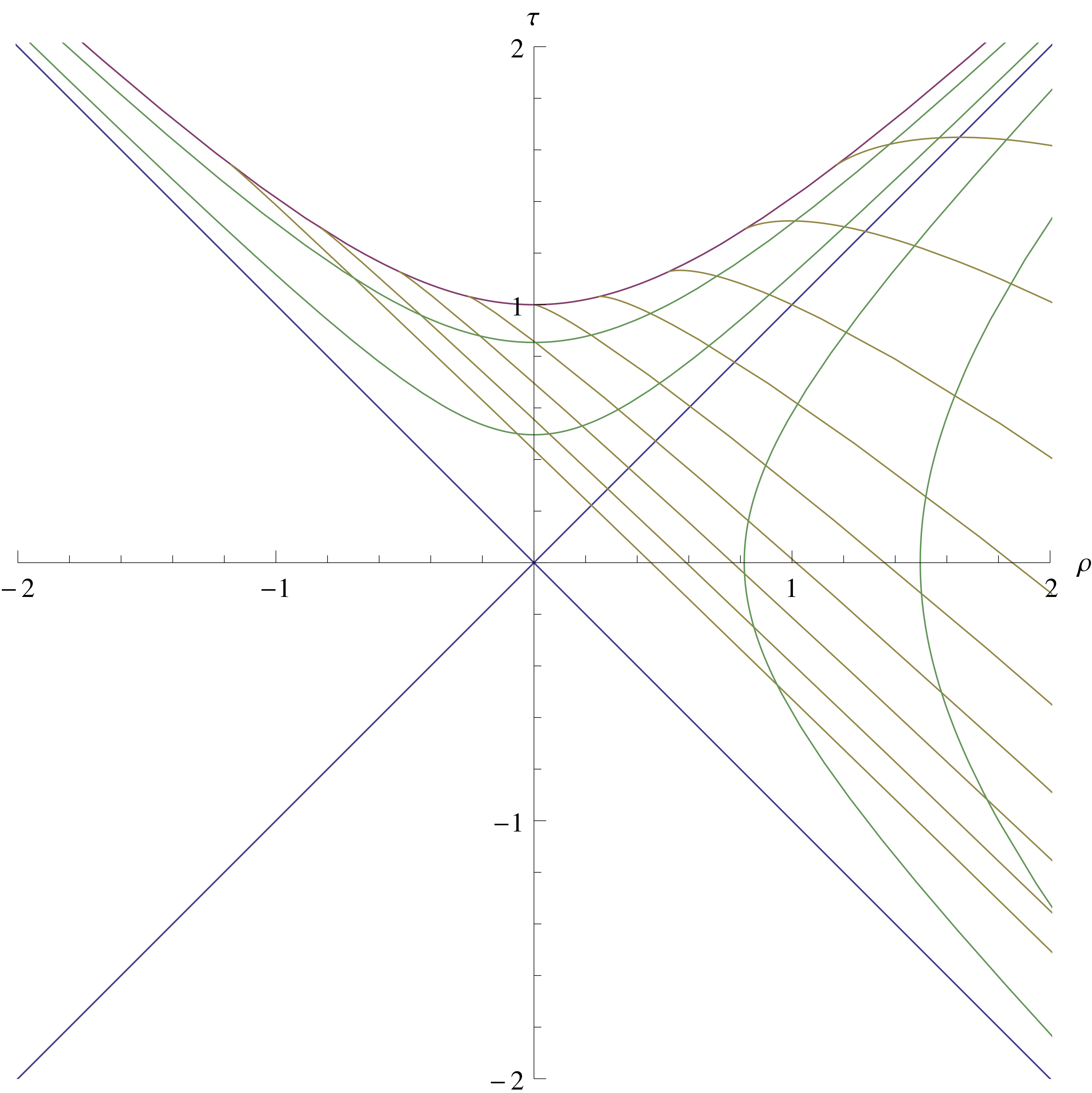
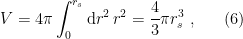
 is much greater than
  (i.e., at late times), one finds [4]
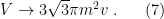
 , for the same reasons we encountered when attempting to define volume above). Since the event horizon is a null-surface, the area is coordinate-invariant; fixing
 can be easily ruled out by considering a black hole merger [1]). And, while it’s a nice consistency check on the universe, it doesn’t really give any insight into why the degrees of freedom are ultimately bounded by the surface area, beyond the necessity-of-curved-space argument above.
 ).
). , i.e., the answer to the yes-or-no question, “does the black hole contain the particle?” This line of reasoning yields
  ; not bad, given that we ignored QFT entirely!
 is the internal energy,
  is the pressure, and
  , and
, and  where
where  is the heat.

 component diverges when
  , which yields an inner (
 ) and outer (
 ) horizon:

 , whereupon

 , one obtains the analogue of the fundamental thermodynamic relation (11) for black holes:
 and
and  are some functions of

 . What about the other terms? As mentioned above, the
  term in (11) corresponds to the work done to the system. And as it turns out, there’s a way of extracting energy from a (charged, rotating) black hole, known as the
  is indeed the analogue of the work that the black hole could perform on some external system; i.e.,
 .
.
 in the expression for the surface gravity
  -dimensional Schwarzschild geometry becomes
  , whereupon the temperature appears as a consequence of the periodicity in Euclidean time; see my
  , which can’t be Fourier transformed back to position space to yield anything localized near the horizon. In other words, near the horizon of a black hole, the meaning of “particles” employed by an external observer breaks down. The fact that black holes can radiate away energy means that if you stop throwing in matter, the black hole will slowly shrink, which seems to contradict Hawking’s area theorem above. The catch is that this theorem relies on the weak energy condition, which states that the matter density along every timelike vector field is non-negative; this is no longer necessarily true once quantum fluctuations are taking into account, so there’s no mathematical contradiction. It does however mean that our formulation of the “second law” of black hole thermodynamics was too naïve: the area (and hence entropy) of a black hole can decrease, but only by emitting Hawking radiation which increases the entropy of the environment by at least as much. This motivates us to introduce the generalized entropy
 (10), and the second is the entropy of the thermal radiation. In full generality, the Second Law of (Black Hole) Thermodynamics is then statement is that the entropy (10) of all black holes, plus the entropy of the rest of the universe, never decreases:
 is negative:
 and hence the heat
  ). Consequently, throwing matter into a black hole to increase its size actually makes it cooler! Conversely, as the black hole emits Hawking radiation, its temperature increases, causing it to emit more radiation, and so on in a feedback loop that causes the black hole to get hotter and hotter as it shrinks away to nothing. (Precisely what happens in the final moments of a black hole’s lifespan is an open question, likely requiring a more developed theory of quantum gravity to answer. Here I’m going to take the majority view that it indeed evaporates away completely). Note that this means that whenever one speaks about black holes thermodynamically, one should use the microcanonical ensemble rather than the canonical ensemble, because the latter is unstable to any quantum fluctuation that changes the mass of the black hole.
 is indeed the physical (thermodynamic) temperature of a single black hole. In this sense, quantum effects were required to resolve the tension between the fact that the information-theoretic interpretation of entropy as the measure of possible internal microstates was applicable to a single black hole — and hence had physical significance — while the temperature had no meaningful physical interpretation in the non-radiating (classical) case. The combination of seemingly disparate regimes in the expression for the entropy (10) is not a coincidence, but represents a truly remarkable unification. It’s perhaps the first thing a successful theory of quantum gravity should be expected to explain.
 . Initially,
  , because our subsystem is empty. As the black hole evaporates,
  (after normalizing): a maximal loss of information has occurred! This is the information paradox in a single graph. In sharp contrast, what quantum mechanics expects to happen is that after the halfway point in the black hole’s lifespan, the late-time radiation starts to purify the early-time radiation we’ve already collected, so the entropy curve should turn around and head back to 0 when the black hole disappears. This is illustrated in the figure below, from Page’s paper [11]. (The lack of symmetry in the upwards and downwards parts is due to the fact that the emission of different particles (in this calculation, just photons and gravitons) affect the change in the black hole entropy and the change in the radiation entropy slightly differently. The turnover isn’t at exactly half the lifetime either, but rather around
  .)
.)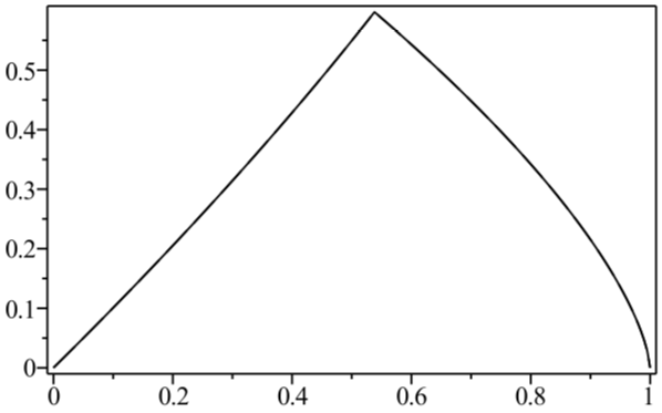
 . For example, in a system with 100 spins, there are
  possible states, so
  and
and  , i.e., the system contains 100 bits of information. One can crudely think of quantum field theory as a continuum theory with a harmonic oscillator at every spacetime point; a single harmonic oscillator already has
  , so one would expect an infinite number of degrees of freedom for any region. However, one can’t localize more than a Planck energy
  into a Planck cube
  without forming a black hole, which provides an ultra-violet (UV) cutoff on the spectrum. And since any finite volume imposes an infra-red (IR) cutoff, we can take the degrees of freedom in field theory to scale like the volume of the region, with one oscillator per Planck cell. In other words, we think of space as a grid with lattice spacing
  ; the total number of oscillators thus scales like the volume
  and
and  . Thus, since
  ,
,  , and we expect entropy to scale with volume just as in classical mechanics.
 , not
, not  , so the energy can’t scale with the volume: the vast majority of the states which QFT would naïvely allow can’t be reached in a gravitational theory, because we form a black hole when we’ve excited only a small fraction of them. The maximum number of states we can excite is
  (in Planck units).
 . If we then collapse that region into a black hole, the Hilbert space dimension would have to suddenly drop to
  . It would then be impossible to recover the initial state from the final state (e.g., after allowing the black hole to evaporate). Thus in order to preserve unitarity, the dimension of the Hilbert space must have been
  ), homogeneous, isotropic space with some average entropy density
 . The proper way to generalize black hole entropy to the sort of bound we want is to recall that the area of the event horizon is a null hypersurface, and it is the formulation in terms of such light-sheets which is consistent with all known examples. This is known as the covariant entropy bound, and states that the entropy on (or rather, contained within) non-expanding light-sheets of some spacetime codimension-2 surface
 ![\displaystyle \langle\Psi|\mathcal{O}(t,\mathbf{x})\tilde{\mathcal{O}}(t',\mathbf{x}')|\Psi\rangle =Z^{-1}\mathrm{tr}\left[e^{-\beta H}\mathcal{O}(t,\mathbf{x})\mathcal{O}(t'+i\beta/2,\mathbf{x}')\right]~, \ \ \ \ \ (1)](https://s0.wp.com/latex.php?latex=%5Cdisplaystyle+%5Clangle%5CPsi%7C%5Cmathcal%7BO%7D%28t%2C%5Cmathbf%7Bx%7D%29%5Ctilde%7B%5Cmathcal%7BO%7D%7D%28t%27%2C%5Cmathbf%7Bx%7D%27%29%7C%5CPsi%5Crangle+%3DZ%5E%7B-1%7D%5Cmathrm%7Btr%7D%5Cleft%5Be%5E%7B-%5Cbeta+H%7D%5Cmathcal%7BO%7D%28t%2C%5Cmathbf%7Bx%7D%29%5Cmathcal%7BO%7D%28t%27%2Bi%5Cbeta%2F2%2C%5Cmathbf%7Bx%7D%27%29%5Cright%5D%7E%2C+%5C+%5C+%5C+%5C+%5C+%281%29&bg=ffffff&fg=000000&s=0&c=20201002)
 and
and 
 in exterior region
  and
and  in exterior region
  . Note that, modulo possible UV divergences at the origin, either half serves as a complete Cauchy slice if we restrict our inquiries to the associated exterior region. But if we wish to reconstruct states in the interior (henceforth just
  , since we don’t care about
  ), then we need the entire slice. Pictorially, one can see this from the fact that only the left-moving modes from region
![\displaystyle \mathrm{d} s^2=\frac{1}{z^2}\left[-h(z)\mathrm{d} t^2+\mathrm{d} z^2+\mathrm{d}\mathbf{x}^2\right]~, \quad\quad h(z)\equiv1-\left(\frac{z}{z_0}\right)^d~. \ \ \ \ \ (3)](https://s0.wp.com/latex.php?latex=%5Cdisplaystyle+%5Cmathrm%7Bd%7D+s%5E2%3D%5Cfrac%7B1%7D%7Bz%5E2%7D%5Cleft%5B-h%28z%29%5Cmathrm%7Bd%7D+t%5E2%2B%5Cmathrm%7Bd%7D+z%5E2%2B%5Cmathrm%7Bd%7D%5Cmathbf%7Bx%7D%5E2%5Cright%5D%7E%2C+%5Cquad%5Cquad+h%28z%29%5Cequiv1-%5Cleft%28%5Cfrac%7Bz%7D%7Bz_0%7D%5Cright%29%5Ed%7E.+%5C+%5C+%5C+%5C+%5C+%283%29&bg=ffffff&fg=000000&s=0&c=20201002)
 , and the horizon is at
  . We work in
  spacetime dimensions, so
  -dimensional vector representing the transverse coordinates. Note that we’ve set the AdS radius to 1. Substituting the usual plane-wave ansatz
 , and hence two linearly independent solutions.
  . Note that we do not impose boundary conditions at the horizon. Naïvely, one might have thought to impose ingoing boundary conditions there; however, as remarked in [1], this precludes the existence of real
  . More intuitively, I think of this as simply the statement that the black hole is evaporating, so we should allow the possibility for outgoing modes as well. (That is, assuming a large black hole in AdS, the black hole is in thermal equilibrium with the surrounding environment, so the outgoing and ingoing fluxes are precisely matched, and it maintains constant size). The expression for
 ![\displaystyle \phi_I(t,\mathbf{x},z)=\int_{\omega>0}\frac{\mathrm{d}\omega\mathrm{d}^{d-1}\mathbf{k}}{\sqrt{2\omega}(2\pi)^d}\,\bigg[ a_{\omega,\mathbf{k}}\,f_{\omega,\mathbf{k}}(t,\mathbf{x},z)+\mathrm{h.c.}\bigg]~, \ \ \ \ \ (5)](https://s0.wp.com/latex.php?latex=%5Cdisplaystyle+%5Cphi_I%28t%2C%5Cmathbf%7Bx%7D%2Cz%29%3D%5Cint_%7B%5Comega%3E0%7D%5Cfrac%7B%5Cmathrm%7Bd%7D%5Comega%5Cmathrm%7Bd%7D%5E%7Bd-1%7D%5Cmathbf%7Bk%7D%7D%7B%5Csqrt%7B2%5Comega%7D%282%5Cpi%29%5Ed%7D%5C%2C%5Cbigg%5B+a_%7B%5Comega%2C%5Cmathbf%7Bk%7D%7D%5C%2Cf_%7B%5Comega%2C%5Cmathbf%7Bk%7D%7D%28t%2C%5Cmathbf%7Bx%7D%2Cz%29%2B%5Cmathrm%7Bh.c.%7D%5Cbigg%5D%7E%2C+%5C+%5C+%5C+%5C+%5C+%285%29&bg=ffffff&fg=000000&s=0&c=20201002)
![\displaystyle [a_{\omega,\mathbf{k}},a^\dagger_{\omega',\mathbf{k}'}]=\delta(\omega-\omega')\delta^{d-1}(\mathbf{k}-\mathbf{k}')~. \ \ \ \ \ (6)](https://s0.wp.com/latex.php?latex=%5Cdisplaystyle+%5Ba_%7B%5Comega%2C%5Cmathbf%7Bk%7D%7D%2Ca%5E%5Cdagger_%7B%5Comega%27%2C%5Cmathbf%7Bk%7D%27%7D%5D%3D%5Cdelta%28%5Comega-%5Comega%27%29%5Cdelta%5E%7Bd-1%7D%28%5Cmathbf%7Bk%7D-%5Cmathbf%7Bk%7D%27%29%7E.+%5C+%5C+%5C+%5C+%5C+%286%29&bg=ffffff&fg=000000&s=0&c=20201002)
![\displaystyle \phi_{III}(t,\mathbf{x},z)=\int_{\omega>0}\frac{\mathrm{d}\omega\mathrm{d}^{d-1}\mathbf{k}}{\sqrt{2\omega}(2\pi)^d}\,\bigg[\tilde a_{\omega,\mathbf{k}}\,g_{\omega,\mathbf{k}}(t,\mathbf{x},z)+\mathrm{h.c.}\bigg]~, \ \ \ \ \ (7)](https://s0.wp.com/latex.php?latex=%5Cdisplaystyle+%5Cphi_%7BIII%7D%28t%2C%5Cmathbf%7Bx%7D%2Cz%29%3D%5Cint_%7B%5Comega%3E0%7D%5Cfrac%7B%5Cmathrm%7Bd%7D%5Comega%5Cmathrm%7Bd%7D%5E%7Bd-1%7D%5Cmathbf%7Bk%7D%7D%7B%5Csqrt%7B2%5Comega%7D%282%5Cpi%29%5Ed%7D%5C%2C%5Cbigg%5B%5Ctilde+a_%7B%5Comega%2C%5Cmathbf%7Bk%7D%7D%5C%2Cg_%7B%5Comega%2C%5Cmathbf%7Bk%7D%7D%28t%2C%5Cmathbf%7Bx%7D%2Cz%29%2B%5Cmathrm%7Bh.c.%7D%5Cbigg%5D%7E%2C+%5C+%5C+%5C+%5C+%5C+%287%29&bg=ffffff&fg=000000&s=0&c=20201002)
 commute with all
  by construction.
![\displaystyle \phi^I_{\mathrm{CFT}}(t,\mathbf{x},z)=\int_{\omega>0}\frac{\mathrm{d}\omega\mathrm{d}^{d-1}\mathbf{k}}{(2\pi)^d}\,\bigg[\mathcal{O}_{\omega,\mathbf{k}}\,f_{\omega,\mathbf{k}}(t,\mathbf{x},z)+\mathcal{O}^\dagger_{\omega,\mathbf{k}}f^*_{\omega,\mathbf{k}}(t,\mathbf{x},z)\bigg]~, \ \ \ \ \ (8)](https://s0.wp.com/latex.php?latex=%5Cdisplaystyle+%5Cphi%5EI_%7B%5Cmathrm%7BCFT%7D%7D%28t%2C%5Cmathbf%7Bx%7D%2Cz%29%3D%5Cint_%7B%5Comega%3E0%7D%5Cfrac%7B%5Cmathrm%7Bd%7D%5Comega%5Cmathrm%7Bd%7D%5E%7Bd-1%7D%5Cmathbf%7Bk%7D%7D%7B%282%5Cpi%29%5Ed%7D%5C%2C%5Cbigg%5B%5Cmathcal%7BO%7D_%7B%5Comega%2C%5Cmathbf%7Bk%7D%7D%5C%2Cf_%7B%5Comega%2C%5Cmathbf%7Bk%7D%7D%28t%2C%5Cmathbf%7Bx%7D%2Cz%29%2B%5Cmathcal%7BO%7D%5E%5Cdagger_%7B%5Comega%2C%5Cmathbf%7Bk%7D%7Df%5E%2A_%7B%5Comega%2C%5Cmathbf%7Bk%7D%7D%28t%2C%5Cmathbf%7Bx%7D%2Cz%29%5Cbigg%5D%7E%2C+%5C+%5C+%5C+%5C+%5C+%288%29&bg=ffffff&fg=000000&s=0&c=20201002)
 which act as creation operators of light primary fields), behaves like a local operator in the bulk. Note that from the perspective of the CFT,
 local bulk fields” is the same.
 living in the left CFT:
![\displaystyle \phi^{III}_{\mathrm{CFT}}(t,\mathbf{x},z)=\int_{\omega>0}\frac{\mathrm{d}\omega\mathrm{d}^{d-1}\mathbf{k}}{(2\pi)^d}\,\bigg[\tilde{\mathcal{O}}_{\omega,\mathbf{k}}\,f_{\omega,\mathbf{k}}(t,\mathbf{x},z)+\tilde{\mathcal{O}}^\dagger_{\omega,\mathbf{k}}f^*_{\omega,\mathbf{k}}(t,\mathbf{x},z)\bigg]~. \ \ \ \ \ (10)](https://s0.wp.com/latex.php?latex=%5Cdisplaystyle+%5Cphi%5E%7BIII%7D_%7B%5Cmathrm%7BCFT%7D%7D%28t%2C%5Cmathbf%7Bx%7D%2Cz%29%3D%5Cint_%7B%5Comega%3E0%7D%5Cfrac%7B%5Cmathrm%7Bd%7D%5Comega%5Cmathrm%7Bd%7D%5E%7Bd-1%7D%5Cmathbf%7Bk%7D%7D%7B%282%5Cpi%29%5Ed%7D%5C%2C%5Cbigg%5B%5Ctilde%7B%5Cmathcal%7BO%7D%7D_%7B%5Comega%2C%5Cmathbf%7Bk%7D%7D%5C%2Cf_%7B%5Comega%2C%5Cmathbf%7Bk%7D%7D%28t%2C%5Cmathbf%7Bx%7D%2Cz%29%2B%5Ctilde%7B%5Cmathcal%7BO%7D%7D%5E%5Cdagger_%7B%5Comega%2C%5Cmathbf%7Bk%7D%7Df%5E%2A_%7B%5Comega%2C%5Cmathbf%7Bk%7D%7D%28t%2C%5Cmathbf%7Bx%7D%2Cz%29%5Cbigg%5D%7E.+%5C+%5C+%5C+%5C+%5C+%2810%29&bg=ffffff&fg=000000&s=0&c=20201002)
![\displaystyle \phi^{II}_{\mathrm{CFT}}(t,\mathbf{x},z)=\int_{\omega>0}\frac{\mathrm{d}\omega\mathrm{d}^{d-1}\mathbf{k}}{(2\pi)^d}\,\bigg[\mathcal{O}_{\omega,\mathbf{k}}\,g^{(1)}_{\omega,\mathbf{k}}(t,\mathbf{x},z)+\tilde{\mathcal{O}}_{\omega,\mathbf{k}}g^{(2)}_{\omega,\mathbf{k}}(t,\mathbf{x},z)+\mathrm{h.c}\bigg]~, \ \ \ \ \ (11)](https://s0.wp.com/latex.php?latex=%5Cdisplaystyle+%5Cphi%5E%7BII%7D_%7B%5Cmathrm%7BCFT%7D%7D%28t%2C%5Cmathbf%7Bx%7D%2Cz%29%3D%5Cint_%7B%5Comega%3E0%7D%5Cfrac%7B%5Cmathrm%7Bd%7D%5Comega%5Cmathrm%7Bd%7D%5E%7Bd-1%7D%5Cmathbf%7Bk%7D%7D%7B%282%5Cpi%29%5Ed%7D%5C%2C%5Cbigg%5B%5Cmathcal%7BO%7D_%7B%5Comega%2C%5Cmathbf%7Bk%7D%7D%5C%2Cg%5E%7B%281%29%7D_%7B%5Comega%2C%5Cmathbf%7Bk%7D%7D%28t%2C%5Cmathbf%7Bx%7D%2Cz%29%2B%5Ctilde%7B%5Cmathcal%7BO%7D%7D_%7B%5Comega%2C%5Cmathbf%7Bk%7D%7Dg%5E%7B%282%29%7D_%7B%5Comega%2C%5Cmathbf%7Bk%7D%7D%28t%2C%5Cmathbf%7Bx%7D%2Cz%29%2B%5Cmathrm%7Bh.c%7D%5Cbigg%5D%7E%2C+%5C+%5C+%5C+%5C+%5C+%2811%29&bg=ffffff&fg=000000&s=0&c=20201002)

 of the CFT set by the mass of the black hole. This implies that correlation functions of operators
  may be computed as thermal expectation values in their (mixed) half of the total Hilbert space, i.e.,
 ![\displaystyle \langle\mathrm{TFD}|\mathcal{O}(t_1,\mathbf{x}_1)\ldots\mathcal{O}(t_n,\mathbf{x}_n)|\mathrm{TFD}\rangle =Z^{-1}_\beta\mathrm{tr}\left[e^{-\beta H}\mathcal{O}(t_1,\mathbf{x}_1)\ldots\mathcal{O}(t_n,\mathbf{x}_n)\right]~. \ \ \ \ \ (13)](https://s0.wp.com/latex.php?latex=%5Cdisplaystyle+%5Clangle%5Cmathrm%7BTFD%7D%7C%5Cmathcal%7BO%7D%28t_1%2C%5Cmathbf%7Bx%7D_1%29%5Cldots%5Cmathcal%7BO%7D%28t_n%2C%5Cmathbf%7Bx%7D_n%29%7C%5Cmathrm%7BTFD%7D%5Crangle+%3DZ%5E%7B-1%7D_%5Cbeta%5Cmathrm%7Btr%7D%5Cleft%5Be%5E%7B-%5Cbeta+H%7D%5Cmathcal%7BO%7D%28t_1%2C%5Cmathbf%7Bx%7D_1%29%5Cldots%5Cmathcal%7BO%7D%28t_n%2C%5Cmathbf%7Bx%7D_n%29%5Cright%5D%7E.+%5C+%5C+%5C+%5C+%5C+%2813%29&bg=ffffff&fg=000000&s=0&c=20201002)
 up to
up to  corrections. The reason this is the “correct” prescription is that it’s the only one which
  ? In the two-sided case, we can simply compute this correlator in the pure state
![\displaystyle \langle\mathrm{TFD}|\mathcal{O}(t_1,\mathbf{x}_1)\ldots\tilde{\mathcal{O}}(t_n,\mathbf{x}_n)|\mathrm{TFD}\rangle =Z^{-1}_\beta\mathrm{tr}\left[e^{-\beta H}\mathcal{O}(t_1,\mathbf{x}_1)\ldots\mathcal{O}_{\omega,\mathbf{k}}(t_n+i\beta/2,\mathbf{x}_n)\right]~, \ \ \ \ \ (15)](https://s0.wp.com/latex.php?latex=%5Cdisplaystyle+%5Clangle%5Cmathrm%7BTFD%7D%7C%5Cmathcal%7BO%7D%28t_1%2C%5Cmathbf%7Bx%7D_1%29%5Cldots%5Ctilde%7B%5Cmathcal%7BO%7D%7D%28t_n%2C%5Cmathbf%7Bx%7D_n%29%7C%5Cmathrm%7BTFD%7D%5Crangle+%3DZ%5E%7B-1%7D_%5Cbeta%5Cmathrm%7Btr%7D%5Cleft%5Be%5E%7B-%5Cbeta+H%7D%5Cmathcal%7BO%7D%28t_1%2C%5Cmathbf%7Bx%7D_1%29%5Cldots%5Cmathcal%7BO%7D_%7B%5Comega%2C%5Cmathbf%7Bk%7D%7D%28t_n%2Bi%5Cbeta%2F2%2C%5Cmathbf%7Bx%7D_n%29%5Cright%5D%7E%2C+%5C+%5C+%5C+%5C+%5C+%2815%29&bg=ffffff&fg=000000&s=0&c=20201002)

 denotes the variational or “action parameters” of the model, so named because they parametrize the action of the brain on its substrate and surroundings. That is, the only way in which the system can change the distribution is by acting to change its sensory inputs. Friston denotes this dependency by
  (with different variables), but as alluded above, I will keep to the present notation to avoid conflating state/parameter spaces.
 is then a map from the space of sensory inputs
  (as modelled by the brain). As in the case of
  . Instead, we construct a new distribution
  for the conditional probability of environment states
 denote the conditional distributions
  is the energy or hamiltonian for the ensemble
  ), and
  is the entropy of
  with the ensemble density
  , where — unlike in the case of
  — we have denoted the variational parameters
  ) get renormalized after marginalizing over some degrees of freedom (here,
 to distinguish this from
  (no vertical bar) denotes that expectation values are computed with respect to the distribution
  as the log-likelihood of sensory inputs given the state of the environment, minus an error term that quantifies how far the brain’s internal model of the world
  for some energy
  and entropy
  ; the reason for this general form involves a
  . As explained above,
  , we can re-arrange the expression for the free energy to isolate this dependence in a single Kullback-Leibler term:
 . This form of the expression shows clearly that minimization with respect to
  in (4) (i.e., zero Kullback-Leibler divergence (2)), whereupon the free energy reduces to the negative log-likelihood of sensory inputs,
 . Since real-world models are generally non-linear in their inputs however, invertibility is not something one expects to encounter in realistic inference machines (i.e., brains). Indeed, our brains evolved under strict energetic and space constraints; there simply isn’t enough processing power to brute-force the problem by using dedicated feed-forward networks for all our recognition needs. The other important exception is when the recognition process is purely deterministic. In this case one replaces
  , so that upon performing the summation, the inferred state
 . Note that the invertible case, (6), corresponds to maximum likelihood estimation (MLE), while the deterministic case (7) corresponds to so-called maximum a posteriori estimation (MAP), the only difference being that the latter includes a weighting based on the prior distribution
  . Neither requires the conditional distribution
  , where 0 is the bottom-most layer and
  denotes sensory data at the corresponding layer; i.e.,
  corresponds to the propagated input signals after all previous levels of processing. Similarly, let
 implicitly depends on the knowledge of the state at all previous levels,
  . For present purposes, this can be identified with
  , since at the bottom-most level of the hierarchy, there’s no difference between the raw sensory data and the inferred state of the world (ignoring whatever intralayer processing might take place). In this (empirical Bayesian) way, the brain self-consistently builds up higher priors from states at lower levels.
 . The total energy function is
 . Note that there are no intra-layer couplings, and that I’ve stacked the layers so that the visible layer
  . There’s an obvious Bayesian parallel here: we low-energy beings don’t have access to complete information about the UV, so the visible units are naturally identified with IR degrees of freedom, and indeed I’ll use these terms interchangeably throughout.
![\displaystyle p(x,y,z)=Z^{-1}e^{-\beta H(x,y,z)}~, \quad\quad Z[\beta]=\prod_{i=1}^n\sum_{x_i=\pm1}\int\!\mathrm{d}^my\mathrm{d}^pz\,e^{-\beta H(x,y,z)}~, \ \ \ \ \ (2)](https://s0.wp.com/latex.php?latex=%5Cdisplaystyle+p%28x%2Cy%2Cz%29%3DZ%5E%7B-1%7De%5E%7B-%5Cbeta+H%28x%2Cy%2Cz%29%7D%7E%2C+%5Cquad%5Cquad+Z%5B%5Cbeta%5D%3D%5Cprod_%7Bi%3D1%7D%5En%5Csum_%7Bx_i%3D%5Cpm1%7D%5Cint%5C%21%5Cmathrm%7Bd%7D%5Emy%5Cmathrm%7Bd%7D%5Epz%5C%2Ce%5E%7B-%5Cbeta+H%28x%2Cy%2Cz%29%7D%7E%2C+%5C+%5C+%5C+%5C+%5C+%282%29&bg=ffffff&fg=000000&s=0&c=20201002)
 , and similarly for
  and
and 
 such that


 and
and  . We therefore obtain
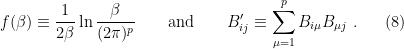

 with respect to this distribution is then
 , we have

 , we then see that the effect of the marginalizing out UV (i.e., hidden) degrees of freedom is to induce higher-order couplings between the IR (i.e., visible) units, with the coefficients of the interaction weighted by the associated cumulant:
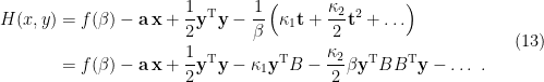
 (the variance) vanish, whereupon (13) reduces to (7) above.
 and
and  . We therefore obtain
![\displaystyle \begin{aligned} p(x)&=Z^{-1}\sqrt{\frac{(2\pi)^m}{\beta\left(1-|B'|\right)}}\mathrm{exp}\left[-\beta\left( f(\beta)-\mathbf{a}\mathbf{x}+\frac{1}{2}\mathbf{x}^\mathrm{T} A\left(\mathbf{1}-B'\right)^{-1}A^\mathrm{T}\mathbf{x}\right)\right]\\ &=Z^{-1}\sqrt{\frac{(2\pi)^m}{\beta\left(1-|B'|\right)}}\mathrm{exp}\left[-\beta\left( f(\beta)-\mathbf{a}\mathbf{x}+\frac{1}{2}\mathbf{x}^\mathrm{T} A'\mathbf{x}\right)\right] \end{aligned} \ \ \ \ \ (15)](https://s0.wp.com/latex.php?latex=%5Cdisplaystyle+%5Cbegin%7Baligned%7D+p%28x%29%26%3DZ%5E%7B-1%7D%5Csqrt%7B%5Cfrac%7B%282%5Cpi%29%5Em%7D%7B%5Cbeta%5Cleft%281-%7CB%27%7C%5Cright%29%7D%7D%5Cmathrm%7Bexp%7D%5Cleft%5B-%5Cbeta%5Cleft%28+f%28%5Cbeta%29-%5Cmathbf%7Ba%7D%5Cmathbf%7Bx%7D%2B%5Cfrac%7B1%7D%7B2%7D%5Cmathbf%7Bx%7D%5E%5Cmathrm%7BT%7D+A%5Cleft%28%5Cmathbf%7B1%7D-B%27%5Cright%29%5E%7B-1%7DA%5E%5Cmathrm%7BT%7D%5Cmathbf%7Bx%7D%5Cright%29%5Cright%5D%5C%5C+%26%3DZ%5E%7B-1%7D%5Csqrt%7B%5Cfrac%7B%282%5Cpi%29%5Em%7D%7B%5Cbeta%5Cleft%281-%7CB%27%7C%5Cright%29%7D%7D%5Cmathrm%7Bexp%7D%5Cleft%5B-%5Cbeta%5Cleft%28+f%28%5Cbeta%29-%5Cmathbf%7Ba%7D%5Cmathbf%7Bx%7D%2B%5Cfrac%7B1%7D%7B2%7D%5Cmathbf%7Bx%7D%5E%5Cmathrm%7BT%7D+A%27%5Cmathbf%7Bx%7D%5Cright%29%5Cright%5D+%5Cend%7Baligned%7D+%5C+%5C+%5C+%5C+%5C+%2815%29&bg=ffffff&fg=000000&s=0&c=20201002)
 . As before, we then define
  such that
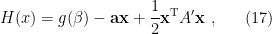

 and
and  are given in (8).
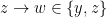 and
and  . This will be of the form (10), where in this case we need to choose
  , so that
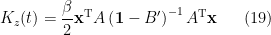
 , the inverse matrix
  is also invariant under the transpose; at this stage of exploration, I’m being quite cavalier about questions of existence). Thus the hamiltonian of visible units may be written
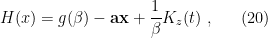
 as above. Since the prior with which these cumulants are computed is again Gaussian, only the second cumulant survives in the expansion, and we indeed recover (17).
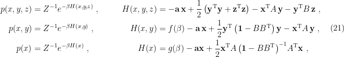
 for
for  for
for 
 between visible (low-energy) degrees of freedom, for example, does not depend on which distribution we use to compute the expectation value, so long as the energy scale thereof is at or above the scale set by the inverse lattice spacing of
 . In this analogy, tracing out
  , which is again one-dimensional. When one speaks of deep “learning” however, one views the network as two-dimensional, and “dynamics” refers to the changing values of the couplings as the network attempts to minimize the cost function. In short, RG lies in the fact that the couplings at each level in (21) encode the
  at this level. Accordingly, [8] instead replace (2) with
 is the so-called reduced (i.e., dimensionless) hamiltonian, cf. the reduced/dimensionless free energy
  in the
  runs over all the degrees of freedom in the theory, which are all UV/hidden variables at the present level.
 already). More confusingly however, their use of the terminology “visible” and “hidden” is backwards with respect to the RG analogy here. In particular, they coarse-grain a block of “visible” units into a single “hidden” unit. For reasons which should by now be obvious, I will instead stick to the natural Bayesian identifications above, in order to preserve the analogy with standard coarse-graining in RG.
 , and then writing the new distribution
  in the canonical form (24). In Bayesian terms, we need to marginalize over the information about
  , except that unlike in my simple example above, we don’t want to make any assumptions about the form of
  . So we instead express the integral — or rather, the discrete sum over lattice sites — in terms of the conditional distribution
  :
:
 ,
,  . Denoting the new dimensionless hamiltonian
  , with
  ,
,  , we therefore have
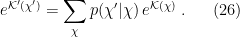
 into a piece containing only intra-block terms,
  (that is, interactions solely among the set of hidden units which is to be coarse-grained into a single visible unit), and a piece containing the remaining, inter-block terms,
  (that is, interactions between different aforementioned sets of hidden units).
 , such that
  (note that since
  , this implies
  degrees of freedom
  per block). To each
  , we associate a visible unit
  , into which the constituent UV variables
  relative to [8]). Then translation invariance implies
 denotes a single intra-block term of the hamiltonian. With this notation in hand, (26) becomes
 , where
  . Given the underlying factorization of the total Hilbert space, we furthermore suppose that the distribution of all intra-block contributions can be written
  , so that
  . This implies that
 into (28), from which the remaining manipulations are straightforward: we identify
 (again by translation invariance), whereupon we have
 . Finally, by taking the log, we obtain
 accounts for the normalization factor
  gives the contribution from the un-marginalized variables
  ; and the log of the expectation values is the contribution from the UV cumulants, cf.
  therein:
 becomes the dimensionless energy
  , so the
  relative to the usual energetic moments in
 , and the expectation values in the generating functions are computed with respect to
 denotes the expectation value for the corresponding distribution. (As a technical caveat: in some cases, the moments — and correspondingly,
  — may not exist, in which case one can resort to the characteristic function instead). By series expanding the exponential, we have
 is the
  , i.e.,

 is the
  :
: 
 is
is ![\displaystyle p_i\equiv p(E_i)=\frac{1}{Z[\beta]}e^{-\beta E_i}~, \quad\quad \sum\nolimits_ip_i=1~. \ \ \ \ \ (6)](https://s0.wp.com/latex.php?latex=%5Cdisplaystyle+p_i%5Cequiv+p%28E_i%29%3D%5Cfrac%7B1%7D%7BZ%5B%5Cbeta%5D%7De%5E%7B-%5Cbeta+E_i%7D%7E%2C+%5Cquad%5Cquad+%5Csum%5Cnolimits_ip_i%3D1%7E.+%5C+%5C+%5C+%5C+%5C+%286%29&bg=ffffff&fg=000000&s=0&c=20201002)
![\displaystyle M_E(t)=\langle e^{tE}\rangle=\sum_i p(E_i)e^{tE_i} =\frac{1}{Z[\beta]}\sum_ie^{-(\beta\!-\!t)E_i} =\frac{Z[\beta-t]}{Z[\beta]}~. \ \ \ \ \ (7)](https://s0.wp.com/latex.php?latex=%5Cdisplaystyle+M_E%28t%29%3D%5Clangle+e%5E%7BtE%7D%5Crangle%3D%5Csum_i+p%28E_i%29e%5E%7BtE_i%7D+%3D%5Cfrac%7B1%7D%7BZ%5B%5Cbeta%5D%7D%5Csum_ie%5E%7B-%28%5Cbeta%5C%21-%5C%21t%29E_i%7D+%3D%5Cfrac%7BZ%5B%5Cbeta-t%5D%7D%7BZ%5B%5Cbeta%5D%7D%7E.+%5C+%5C+%5C+%5C+%5C+%287%29&bg=ffffff&fg=000000&s=0&c=20201002)
![{Z[\beta]}](https://s0.wp.com/latex.php?latex=%7BZ%5B%5Cbeta%5D%7D&bg=ffffff&fg=000000&s=0&c=20201002) is not the moment generating function, but there’s clearly a close relationship between the two. Rather, the precise statement is that the moment generating function
is not the moment generating function, but there’s clearly a close relationship between the two. Rather, the precise statement is that the moment generating function  is the ratio of two partition functions at inverse temperatures
  and
and ![\displaystyle \langle E^n\rangle=M^{(n)}(t)\Big|_{t=0} =\frac{1}{Z[\beta]}\frac{\partial^n}{\partial t^n}Z[\beta\!-\!t]\bigg|_{t=0} =(-1)^n\frac{Z^{(n)}[\beta\!-\!t]}{Z[\beta]}\bigg|_{t=0} =(-1)^n\frac{Z^{(n)}[\beta]}{Z[\beta]}~. \ \ \ \ \ (8)](https://s0.wp.com/latex.php?latex=%5Cdisplaystyle+%5Clangle+E%5En%5Crangle%3DM%5E%7B%28n%29%7D%28t%29%5CBig%7C_%7Bt%3D0%7D+%3D%5Cfrac%7B1%7D%7BZ%5B%5Cbeta%5D%7D%5Cfrac%7B%5Cpartial%5En%7D%7B%5Cpartial+t%5En%7DZ%5B%5Cbeta%5C%21-%5C%21t%5D%5Cbigg%7C_%7Bt%3D0%7D+%3D%28-1%29%5En%5Cfrac%7BZ%5E%7B%28n%29%7D%5B%5Cbeta%5C%21-%5C%21t%5D%7D%7BZ%5B%5Cbeta%5D%7D%5Cbigg%7C_%7Bt%3D0%7D+%3D%28-1%29%5En%5Cfrac%7BZ%5E%7B%28n%29%7D%5B%5Cbeta%5D%7D%7BZ%5B%5Cbeta%5D%7D%7E.+%5C+%5C+%5C+%5C+%5C+%288%29&bg=ffffff&fg=000000&s=0&c=20201002)
 ). Of course, this is simply a more formal expression for the usual thermodynamic expectation values. The first moment of energy, for example, is
![\displaystyle \langle E\rangle= -\frac{1}{Z[\beta]}\frac{\partial Z[\beta]}{\partial\beta} =\frac{1}{Z[\beta]}\sum_i E_ie^{-\beta E_i} =\sum_i E_i\,p_i~, \ \ \ \ \ (9)](https://s0.wp.com/latex.php?latex=%5Cdisplaystyle+%5Clangle+E%5Crangle%3D+-%5Cfrac%7B1%7D%7BZ%5B%5Cbeta%5D%7D%5Cfrac%7B%5Cpartial+Z%5B%5Cbeta%5D%7D%7B%5Cpartial%5Cbeta%7D+%3D%5Cfrac%7B1%7D%7BZ%5B%5Cbeta%5D%7D%5Csum_i+E_ie%5E%7B-%5Cbeta+E_i%7D+%3D%5Csum_i+E_i%5C%2Cp_i%7E%2C+%5C+%5C+%5C+%5C+%5C+%289%29&bg=ffffff&fg=000000&s=0&c=20201002)
![\displaystyle K_E(t)=\ln\langle e^{tE}\rangle=\ln Z[\beta\!-\!t]-\ln Z[\beta]~. \ \ \ \ \ (10)](https://s0.wp.com/latex.php?latex=%5Cdisplaystyle+K_E%28t%29%3D%5Cln%5Clangle+e%5E%7BtE%7D%5Crangle%3D%5Cln+Z%5B%5Cbeta%5C%21-%5C%21t%5D-%5Cln+Z%5B%5Cbeta%5D%7E.+%5C+%5C+%5C+%5C+%5C+%2810%29&bg=ffffff&fg=000000&s=0&c=20201002)
![\displaystyle \begin{aligned} K^{(1)}(t)\big|_{t=0}&=-\frac{Z'[\beta]}{Z[\beta]}=\langle E\rangle~,\\ K^{(2)}(t)\big|_{t=0}&=\frac{Z''[\beta]}{Z[\beta]}-\left(\frac{Z'[\beta]}{Z[\beta]}\right)^2=\langle E^2\rangle-\langle E\rangle^2\\ K^{(3)}(t)\big|_{t=0}&=-2\left(\frac{Z'[\beta]}{Z[\beta]}\right)^3+3\frac{Z'[\beta]Z''[\beta]}{Z[\beta]^2}-\frac{Z^{(3)}[\beta]}{Z[\beta]}\\ &=-2\langle E\rangle^3+3\langle E\rangle\langle E^2\rangle-\langle E^3\rangle =-\left\langle\left( E-\langle E\rangle\right)^3\right\rangle~. \end{aligned} \ \ \ \ \ (11)](https://s0.wp.com/latex.php?latex=%5Cdisplaystyle+%5Cbegin%7Baligned%7D+K%5E%7B%281%29%7D%28t%29%5Cbig%7C_%7Bt%3D0%7D%26%3D-%5Cfrac%7BZ%27%5B%5Cbeta%5D%7D%7BZ%5B%5Cbeta%5D%7D%3D%5Clangle+E%5Crangle%7E%2C%5C%5C+K%5E%7B%282%29%7D%28t%29%5Cbig%7C_%7Bt%3D0%7D%26%3D%5Cfrac%7BZ%27%27%5B%5Cbeta%5D%7D%7BZ%5B%5Cbeta%5D%7D-%5Cleft%28%5Cfrac%7BZ%27%5B%5Cbeta%5D%7D%7BZ%5B%5Cbeta%5D%7D%5Cright%29%5E2%3D%5Clangle+E%5E2%5Crangle-%5Clangle+E%5Crangle%5E2%5C%5C+K%5E%7B%283%29%7D%28t%29%5Cbig%7C_%7Bt%3D0%7D%26%3D-2%5Cleft%28%5Cfrac%7BZ%27%5B%5Cbeta%5D%7D%7BZ%5B%5Cbeta%5D%7D%5Cright%29%5E3%2B3%5Cfrac%7BZ%27%5B%5Cbeta%5DZ%27%27%5B%5Cbeta%5D%7D%7BZ%5B%5Cbeta%5D%5E2%7D-%5Cfrac%7BZ%5E%7B%283%29%7D%5B%5Cbeta%5D%7D%7BZ%5B%5Cbeta%5D%7D%5C%5C+%26%3D-2%5Clangle+E%5Crangle%5E3%2B3%5Clangle+E%5Crangle%5Clangle+E%5E2%5Crangle-%5Clangle+E%5E3%5Crangle+%3D-%5Cleft%5Clangle%5Cleft%28+E-%5Clangle+E%5Crangle%5Cright%29%5E3%5Cright%5Crangle%7E.+%5Cend%7Baligned%7D+%5C+%5C+%5C+%5C+%5C+%2811%29&bg=ffffff&fg=000000&s=0&c=20201002)
![\displaystyle K_E(\beta)\equiv-\ln Z[\beta] \qquad\implies\qquad \kappa_n=(-1)^{n-1}K_E^{(n)}(\beta)~, \ \ \ \ \ (12)](https://s0.wp.com/latex.php?latex=%5Cdisplaystyle+K_E%28%5Cbeta%29%5Cequiv-%5Cln+Z%5B%5Cbeta%5D+%5Cqquad%5Cimplies%5Cqquad+%5Ckappa_n%3D%28-1%29%5E%7Bn-1%7DK_E%5E%7B%28n%29%7D%28%5Cbeta%29%7E%2C+%5C+%5C+%5C+%5C+%5C+%2812%29&bg=ffffff&fg=000000&s=0&c=20201002)
![{F[\beta]=-\beta^{-1}\ln Z[\beta]}](https://s0.wp.com/latex.php?latex=%7BF%5B%5Cbeta%5D%3D-%5Cbeta%5E%7B-1%7D%5Cln+Z%5B%5Cbeta%5D%7D&bg=ffffff&fg=000000&s=0&c=20201002) ? Given the form (12), one sees that they’re essentially one and the same, up to a factor of
? Given the form (12), one sees that they’re essentially one and the same, up to a factor of 
 is the Boltzmann distribution (6). However, the factor of
  — that serves as the cumulant generating function for the distribution. We’ll return to this idea momentarily, cf. (21) below.
![\displaystyle Z[J]=\mathcal{N}\int\mathcal{D}\phi\,\exp\left\{i\!\int\!\mathrm{d}^dx\left[\mathcal{L}(\phi,\partial\phi)+J(x)\phi(x)\right]\right\} \ \ \ \ \ (14)](https://s0.wp.com/latex.php?latex=%5Cdisplaystyle+Z%5BJ%5D%3D%5Cmathcal%7BN%7D%5Cint%5Cmathcal%7BD%7D%5Cphi%5C%2C%5Cexp%5Cleft%5C%7Bi%5C%21%5Cint%5C%21%5Cmathrm%7Bd%7D%5Edx%5Cleft%5B%5Cmathcal%7BL%7D%28%5Cphi%2C%5Cpartial%5Cphi%29%2BJ%28x%29%5Cphi%28x%29%5Cright%5D%5Cright%5C%7D+%5C+%5C+%5C+%5C+%5C+%2814%29&bg=ffffff&fg=000000&s=0&c=20201002)
 :
:![\displaystyle G^{(n)}(x_1,\ldots,x_n)=\frac{1}{i^n}\frac{\delta^nZ[J]}{\delta J(x_1)\ldots\delta J(x_n)}\bigg|_{J=0}~, \ \ \ \ \ (15)](https://s0.wp.com/latex.php?latex=%5Cdisplaystyle+G%5E%7B%28n%29%7D%28x_1%2C%5Cldots%2Cx_n%29%3D%5Cfrac%7B1%7D%7Bi%5En%7D%5Cfrac%7B%5Cdelta%5EnZ%5BJ%5D%7D%7B%5Cdelta+J%28x_1%29%5Cldots%5Cdelta+J%28x_n%29%7D%5Cbigg%7C_%7BJ%3D0%7D%7E%2C+%5C+%5C+%5C+%5C+%5C+%2815%29&bg=ffffff&fg=000000&s=0&c=20201002)
 is fixed by demanding that in the absence of sources, we should recover the vacuum expectation value, i.e.,
 ![{Z[0]=\langle0|0\rangle=1}](https://s0.wp.com/latex.php?latex=%7BZ%5B0%5D%3D%5Clangle0%7C0%5Crangle%3D1%7D&bg=ffffff&fg=000000&s=0&c=20201002) . In the language of Feynman diagrams, the Green function contains all possible graphs — both connected and disconnected — that contribute to the corresponding transition amplitude. For example, the 4-point correlator of
. In the language of Feynman diagrams, the Green function contains all possible graphs — both connected and disconnected — that contribute to the corresponding transition amplitude. For example, the 4-point correlator of  theory contains, at first order in the coupling, a disconnected graph consisting of two Feynman propagators, another disconnected graph consisting of a Feynman propagator and a 1-loop diagram, and an irreducible graph consisting of a single 4-point vertex. But only the last of these contributes to the scattering process, so it’s often more useful to work with the generating function for connected diagrams only,
 ![\displaystyle W[J]=-i\ln Z[J]~, \ \ \ \ \ (16)](https://s0.wp.com/latex.php?latex=%5Cdisplaystyle+W%5BJ%5D%3D-i%5Cln+Z%5BJ%5D%7E%2C+%5C+%5C+%5C+%5C+%5C+%2816%29&bg=ffffff&fg=000000&s=0&c=20201002)
 :
:![\displaystyle G_c^{(n)}(x_1,\ldots,x_n)=\frac{1}{i^{n-1}}\frac{\delta^nW[J]}{\delta J(x_1)\ldots\delta J(x_n)}\bigg|_{J=0}~. \ \ \ \ \ (17)](https://s0.wp.com/latex.php?latex=%5Cdisplaystyle+G_c%5E%7B%28n%29%7D%28x_1%2C%5Cldots%2Cx_n%29%3D%5Cfrac%7B1%7D%7Bi%5E%7Bn-1%7D%7D%5Cfrac%7B%5Cdelta%5EnW%5BJ%5D%7D%7B%5Cdelta+J%28x_1%29%5Cldots%5Cdelta+J%28x_n%29%7D%5Cbigg%7C_%7BJ%3D0%7D%7E.+%5C+%5C+%5C+%5C+%5C+%2817%29&bg=ffffff&fg=000000&s=0&c=20201002)
![{Z[J]=\exp{i W[J]}}](https://s0.wp.com/latex.php?latex=%7BZ%5BJ%5D%3D%5Cexp%7Bi+W%5BJ%5D%7D%7D&bg=ffffff&fg=000000&s=0&c=20201002) , is not obvious at first glance, but it is a basic exercise in one’s first QFT course to show that the coefficients of various diagrams indeed work out correctly by simply Taylor expanding the exponential
, is not obvious at first glance, but it is a basic exercise in one’s first QFT course to show that the coefficients of various diagrams indeed work out correctly by simply Taylor expanding the exponential  . In the example of
  into
into  with
with  . The factor of
  in (16) goes away in Euclidean signature, whereupon we see that
 ![{Z[J]}](https://s0.wp.com/latex.php?latex=%7BZ%5BJ%5D%7D&bg=ffffff&fg=000000&s=0&c=20201002) is analogous to
is analogous to ![{W[J]}](https://s0.wp.com/latex.php?latex=%7BW%5BJ%5D%7D&bg=ffffff&fg=000000&s=0&c=20201002) is analogous to
is analogous to ![{\beta F[\beta]}](https://s0.wp.com/latex.php?latex=%7B%5Cbeta+F%5B%5Cbeta%5D%7D&bg=ffffff&fg=000000&s=0&c=20201002) — and hence plays the role of the cumulant generating function in the form (12).
— and hence plays the role of the cumulant generating function in the form (12). -point correlator
  becomes
 are zero. (For a probabilist’s exposition on the relationship between cumulants and connectivity, see the first of three lectures by Novak and LaCroix [1], which takes a more graph-theoretic approach).
![{\Gamma[\phi]}](https://s0.wp.com/latex.php?latex=%7B%5CGamma%5B%5Cphi%5D%7D&bg=ffffff&fg=000000&s=0&c=20201002) , defined as the Legendre transform of
, defined as the Legendre transform of ![\displaystyle \Gamma[\phi]=W[J]-\int\!\mathrm{d} x\,J(x)\phi(x)~. \ \ \ \ \ (19)](https://s0.wp.com/latex.php?latex=%5Cdisplaystyle+%5CGamma%5B%5Cphi%5D%3DW%5BJ%5D-%5Cint%5C%21%5Cmathrm%7Bd%7D+x%5C%2CJ%28x%29%5Cphi%28x%29%7E.+%5C+%5C+%5C+%5C+%5C+%2819%29&bg=ffffff&fg=000000&s=0&c=20201002)

 (13) obscures the duality between the properly dimensionless quantities
  . From this perspective, it is more natural to work with
  instead, in which case we have both an elegant expression for the duality in terms of the Legendre transform, and a precise identification of the dimensionless free energy with the cumulant generating function (12):
 represent the outcome of some measurement or operation (e.g., a coin toss); then the mean after

 is the aforementioned rate function. The formal similarity with the partition function in terms of the effective action,
  , is obvious, though the precise dictionary between the two languages is not. I suspect that a precise translation between the two languages — physics and information theory — can be made here as well, in which the increasing rarity of events as one moves along the tail of the distribution correspond to increasingly high-order corrections to the quantum effective action, but I haven’t worked this out in detail.