If you’ve been following the arXiv, or keeping abreast of developments in high-energy theory more broadly, you may have noticed that the longstanding black hole information paradox seems to have entered a new phase, instigated by a pair of papers [1,2] that appeared simultaneously in the summer of 2019. Over 200 subsequent papers have since appeared on the subject of “islands”—subleading saddles in the gravitational path integral that enable one to compute the Page curve, the signature of unitary black hole evaporation. Due to my skepticism towards certain aspects of these constructions (which I’ll come to below), my brain has largely rebelled against boarding this particular hype train. However, I was recently asked to explain them at the HET group seminar here at Nordita, which provided the opportunity (read: forced me) to prepare a general overview of what it’s all about. Given the wide interest and positive response to the talk, I’ve converted it into the present post to make it publicly available.

Well, most of it: during the talk I spent some time introducing black hole thermodynamics and the information paradox. Since I’ve written about these topics at length already, I’ll simply refer you to those posts for more background information. If you’re not already familiar with firewalls, I suggest reading them first before continuing. It’s ok, I’ll wait.

Done? Great; let me summarize the pre-island state of affairs with the following two images, which I took from the post-island review [3] (also worth a read):

On the left is the Penrose diagram for an evaporating black hole in asymptotically Minkowski space. We suppose the black hole formed from some initially pure state of matter (in this case, a star, denoted in yellow), and evaporates completely via the production of Hawking radiation (represented by the pairs of squiggly lines). The key thing to note is that the Hawking modes are pairwise entangled: the interior partner is trapped behind the horizon and eventually hits the singularity, while the exterior partner is free to escape to infinity as Hawking radiation. An observer who remains far outside the black hole and attempts to collect this radiation will then find the final state to be highly mixed (in fact, almost thermal), since along any timeslice (the green slices), she only has access to the modes outside the horizon. But since we took the initial state to be pure (entropy ), that violates unitarity; this is the information paradox in a nutshell.

The evaporation process is depicted in the right figure, which schematically plots various relevant entropies over time. On the one hand, the Bekenstein-Hawking entropy of the black hole starts at some large value given by the surface area, and steadily decreases as the hole evaporates (orange curve). Meanwhile, the entropy of the radiation starts at zero, and then steadily increases over time as more and more modes are collected. This is the result given in Hawking’s original calculation [4], represented by the green curve. The expectation from unitarity is that the entropy of the radiation should instead follow the so-called Page curve, shown in purple. The idea is that at around the halfway point — more accurately, the point at which the entropy of the radiation equals the entropy of the horizon — the emitted modes start to purify the previously-collected radiation, so the entropy starts to decrease. Eventually, when the black hole has completely evaporated and all the “information” has been emitted, the radiation should again be in a pure state with .

In a nutshell, the island formula is a prescription for computing the entropy of the radiation in such a way as to reproduce the Page curve. The claim is that instead of naïvely tracing-out the black hole interior, one should assign the radiation the generalized entropy

where is the minimal quantum extremal surface (QES), and is the semi-classical entropy of matter fields on the union of (the exterior portion of the Cauchy slice where the radiation is collected) and (a new portion of the Cauchy slice that lies inside the black hole). The next section of this post will trace a quasi-historical route through the various ingredients leading up to this formula, in an attempt to provide some context for an expression that otherwise appears rather out of the blue. Those who work on bulk reconstruction in AdS/CFT can probably skip to “Some Flat Space Intuition” below.

Quantum Extremal Surfaces

While the Penrose diagram above (and most of those below) depicts a black hole in asymptotically flat space, the island formula (1) is properly formulated in AdS/CFT, which is where our story begins. In the interest of making this maximally accessible, let’s start at the beginning with my favourite picture of the hyperbolic disc, courtesy of M. C. Escher:

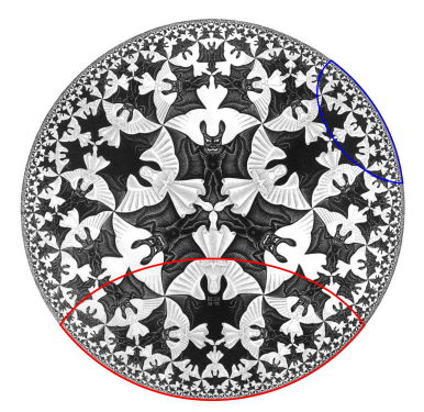
Here we have a gravitational theory living in the bulk anti-de Sitter (AdS) space, which is dual to some conformal field theory (CFT) living on the asymptotic boundary. (Since this picture is necessarily embedded in flat space, the hyperbolic nature of the bulk manifests in the fact that the devils are all the same size). Inherent in the nature of a duality is that every element on one side has an equivalent element on the other, and a major research area in AdS/CFT is completing the so-called holographic dictionary that relates them. One of the major lessons of the past decade is that entanglement entropy appears to play a significant role in this mapping. In particular, the Ryu-Takayanagi formula [5] states that the von Neumann entropy of a boundary subregion — e.g., the blue or red boundary segments I’ve drawn over the image above — is given by the area of the co-dimension 2 minimal surface in the bulk anchored to the boundary of said region that satisfies the homology constraint (see below) — e.g., the blue or red arcs extending towards the center — called the Ryu-Takayanagi or RT surface. More generally, the idea is that all of the physics within the enclosed bulk region can be described by operators living in the corresponding boundary segment (more precisely, its causal domain of dependence).

The most salient aspect of this proposal for our purposes is that it has precisely the same form as the Bekenstein-Hawking entropy, i.e.,

where is the boundary subregion, and the area is that of the corresponding minimal RT surface (in AdS, a spacelike geodesic) in the bulk. As discussed in the post on black hole thermodynamics however, the Bekenstein-Hawking entropy is inadequate if one wishes to capture semi-classical effects, i.e., quantum fields propagating on the black hole (or AdS) background. Rather, one must consider the generalized entropy of the black hole plus radiation:

where for consistency I’ve denoted the entropy of the radiation . As shown in [6], precisely the same formal expression appears in AdS/CFT when one takes into consideration one-loop corrections from quantum fields living between the bulk minimal surface and the corresponding boundary subregion. Intuitively, this plays the same role as the radiation in the black hole picture: just as the external observer must include both the area term and the radiation if she wishes to properly account for the entropy, so too does the entropy of the CFT subregion capture both the area contribution and the entropy of all the enclosed bulk fields.

Formally, the generalized entropy (3) is exactly the quantity that appears in the innermost brackets in the island formula (1), subject to the details of how one selects what semi-classical entropy to compute—more on this below. What about the condition? This has roots in the Ryu-Takayanagi prescription as well, in the form of the aforementioned homology constraint required for computing holographic entanglement entropy. This is discussed at length in [7], and conceptually summarized by the following images therefrom:

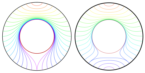
This is again the hyperbolic disc, but with a large AdS black hole whose horizon is demarcated by the inner circle. Now imagine starting with a small boundary subregion at the top of the image, whose corresponding bulk RT surface is drawn in red. As we make this region progressively larger, the RT surface lies deeper and deeper into the bulk—this is represented by the shading from red towards violet. Since the surfaces are defined geometrically, they are sensitive to the presence of the black hole, and get deformed around it as we include more and more of the boundary in the subregion under consideration. Eventually the subregion includes the entire boundary, and the corresponding RT surface is the violet one in the left image. For BTZ black holes, that’s it.

In higher dimensions however, there’s a second RT surface that becomes relevant when the subregion reaches a certain size. Consider the right image, at the point where the RT surface for the subregion is blue. The old solution is the RT surface that loops back around the black hole, on the same side as the boundary subregion. The new solution is the RT surface that connects these same two boundary points on the opposite (that is, lower) side of the black hole, plus a piece that wraps around the horizon itself. The horizon is included because the RT prescription requires the surface to be homologous to the boundary (crudely speaking, we wrap a second piece around the black hole in order to excise the hole from the manifold, so that the solution remains in the same homology class. The fact that one must consider disconnected surfaces may seem rather bizarre, but there’s nothing intrinsically pathological about it; see [7] for more discussion and additional references on the homology constraint in this context). One can see visually that when the boundary subregion reaches a certain size, the combined length of these two pieces will be smaller than the length of the old RT surface that has to go around the black hole the long way. A priori, we now have an ambiguity in which bulk entity we identify with the entropy of the boundary subregion, which is resolved by the requirement that we choose the minimum among all such choices. (While I’m unaware of a satisfactory physical explanation for this, it appears necessary in order for the generalized entropy to satisfy subadditivity [8]). Therefore, as the size of the boundary subregion is continuously increased, a discontinuous (i.e., non-perturbative) switchover occurs to the new minimal surface. As we shall see, a similar switchover plays a crucial role in the island computation of the Page curve.

Now, a quantum extremal surface (QES) is a seemingly mild correction to the above prescription, whereby the semi-classical contribution is taken into account when selecting the surface itself. That is, in the above RT prescription, we selected the minimal surface (which fixes the area term in (3)), and then added the entropy of all the matter fields living between that fixed surface and the boundary (the second term in (3)). As argued in [9] however, the correct procedure is to instead find the surface such that the combination of both terms is extremized, which defines the QES, denoted (equivalently, may be defined as a marginally trapped surface in both the past and future null directions, ). There’s nothing “quantum” about the surface itself (it’s still purely geometrical), the name merely reflects the fact that the quantum corrections to the leading area term (that is, ) are taken into account when determining the surface’s location. The classical extremal surface (i.e., RT without quantum corrections, (2)) is then recovered in the limit . Generically however, the QES will be spacelike separated from its classical counterpart, so that it probes more deeply into the bulk. This is illustrated by the picture below, from [9], where denotes the causal surface for the boundary subregion (which is equivalent to the classical extremal surface in vacuum spacetimes), and the causal domain of dependence in both the bulk (the wedge ) and the boundary (the domain ) are shown by the shaded green region. The QES shares the same boundary points , but extends more deeply into the bulk, since it is defined by extremizing both the area and the quantum corrections together.

In most cases, the difference between the QES and its classical counterpart is relatively small. However, the remarkable feature uncovered in [1,2] is that this can sometimes be quite large, and furthermore, that the QES can sometimes lie deep inside the black hole. This is in sharp contrast to the classical RT surfaces discussed above: as one can see in those rainbow images from [7], they never reach beyond the horizon. (In fact, this appears to be a limitation of all such classical probes, as my colleagues and I analyzed in detail when I was a PhD student [10]: one can get exponentially close to the horizon in some cases, but no better. The corresponding “holographic shadows” seem to represent a puzzle for holographers, since — as per AdS/CFT being a duality — the boundary must have a complete and equivalent description of the physics in the bulk, including the black hole).

These two elements — the minimality requirement, and the ability of QESs to probe behind horizons — are the key to islands.

Some Flat Space Intuition

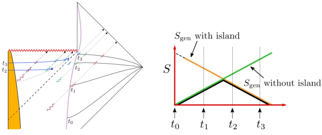
Let us set holography aside for the moment, and return to the flat space Penrose diagram for an evaporating black hole we introduced above. The review [3] does a great job painting an intuitive picture of how the QES changes the story. In particular, the various ingredients in (1) are shown in the following Penrose diagram:

The basic idea is as follows: suppose one is an external observer moving along the timelike trajectory given by the dashed purple line, who collects Hawking radiation that escapes to infinity. The latter comprises the semi-classical entropy along , the “radiation” subset of the Cauchy slice . However, the novelty in the island formula is the claim that this does not comprise the full contribution to the semi-classical entropy . Rather, one must also include the interior modes along the “island” subregion of the Cauchy slice, . The latter is defined as the region between the origin and the QES denoted by the blue point (marked in the image).

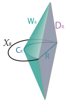
To understand why this QES appears, consider the following diagram, again from [3]. Suppose we fix a Cauchy slice at some point in the evaporation process (say, time in the figure), start with the candidate QES right on the horizon, and imagine moving it along the slice to find the extremum. Initially, the portion of the Cauchy slice denoted captures all interior modes, some of which have not yet been included in the radiation , so has some finite value. As we move the surface inwards along the Cauchy slice, effectively shrinking , we stop capturing some of the unpaired modes, so decreases. Eventually however, we start losing modes whose partners are included in the radiation, at which point will begin to increase. Meanwhile, the area monotonically decreases. The candidate surface becomes a QES at the point where the decrease in the area term precisely cancels the increase in the semi-classical term .

If we repeat this process along an earlier Cauchy slice however, the picture is quite different. Before any radiation has been emitted, shrinking simply decreases the semi-classical entropy as well as the area, so the QES becomes a vanishing surface at the origin. In this case, as we then move forwards in time, all of the entropy (1) comes from the radiation captured in , between the observer’s worldline and infinity.

We thus have two possible choices for the QES that appears in the island formula (1): the vanishing surface at the origin, and the non-vanishing surface that appears at later times. In analogy with the RT prescription above, we are instructed to select whichever yields lower generalized entropy at any given time. Starting at in the Penrose diagram above, we have only the vanishing surface, so our plot of the generalized entropy as the black hole evaporates starts looking exactly as it did in the original story summarized at the beginning of this post: since , the only contribution to the generalized entropy is , which increases monotonically as more and more modes are collected. In particular, as explained above, the issue is that these modes are pairwise entangled with partners trapped behind the horizon. The more unpaired modes we collect, the larger the entropy becomes; thus if we use the vanishing surface , we get the green curve in the schematic plot.

Shortly after the black hole starts to evaporate however, the second, non-vanishing QES appears some distance inside the horizon. The corresponding area contribution is initially very large, but steadily decreases as the hole evaporates. Crucially, the semi-classical contribution also declines, since we count modes in the union , which enables us to capture both partners (see the colored pairs of modes in the Penrose diagram). Using this QES for the generalized entropy then gives us the orange curve in the plot.

Since we’re instructed to always use the minimum QES, a switchover analogous to that we discussed in the context of RT surfaces thus occurs at the Page time: at this point, the area of the non-empty QES (which dominates over the corresponding semi-classical contribution) equals the semi-classical contribution from the empty QES. We therefore follow the black curve in the plot, which is the sought-after Page curve, where the change from an increasing (green) to decreasing (orange) entropy corresponds to a non-perturbative shift in the location of the minimal QES. In this way, the island formula obtains a result for the generalized entropy consistent with our expectations from unitarity.

However, while the exposition above paints a nice intuitive picture, it’s ultimately just a cartoon, and leaves many physical aspects unexplained—for example, how the interior “island” is able to purify the radiation, or the dependence of (the location of) on the observer’s worldline (since the latter controls the size of ). As mentioned at the beginning of this flat space interlude, the island prescription is properly formulated in AdS/CFT, which is the setting in which we actually know how to perform these computations (indeed, it has not been shown that the crucial QES even exists in asymptotically Minkowski space). Even then, analytical computations to date have only been performed in lower-dimensional toy models. These have the powerful advantage of allowing one finer control over various technical aspects of the construction, and also provide the setting in which the claimed derivations of the island formula (1) via the replica trick are performed [11,12]. However, as alluded at the beginning of this post, these rely on some assumptions that I personally find unphysical, or at least insufficiently justified given the current state of our knowledge. So let’s now return to AdS/CFT, and discuss these in a bit more detail.

Just drink the Kool-Aid

There are two main stumbling blocks that must be overcome for the picture we’ve painted above to work:

1. Large black holes in AdS don’t evaporate.
2. The identification of the island with the radiation is ultimately imposed by hand.

The first of these is due to the fact that large AdS black holes, unlike their flat-space counterparts, are microcanonically stable: they have , rather than . Intuitively, AdS acts like a box that reflects the radiation back into the black hole, allowing it to reach thermal equilibrium with the ambient spacetime. Consequently, since the black hole never evaporates, there’s no Page curve to speak of in the first place: it emits radiation until it reaches equilibrium, and then contentedly bathes in it for all eternity.

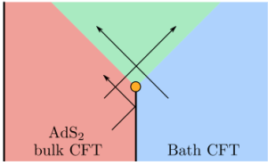
To circumvent this, [1,2] coupled the system to an auxiliary reservoir in order to force the black hole to evaporate. This is illustrated by the following figure from [2], in which a coupling between the asymptotic boundary and a previously-independent CFT that acts as a bath is turned on at the time indicated by the orange dot. Prior to this, radiation from the AdS black hole (not shown) is reflected back into the bulk as explained above; afterwards however, it is able to propagate out of the bulk and into the bath CFT, which they take to live in Minkowski space. This effectively changes the asymptotic structure so that the black hole evaporates by the collection of radiation in this auxiliary reservoir.

This is approximately the point at which I get off the metaphorical train. In particular, insofar as AdS/CFT is a duality between equivalent descriptions of the same system, not two systems that interact at some physical boundary, the so-called “absorbing boundary conditions” [1,2] claim when performing this operation do not appear to me to be valid. Another way to express this underlying point is that it is incorrect to treat the bulk and boundary as akin to tensor factorizations of a single all-encompassing Hilbert space. Rather, the radiation — which carries some finite energy — has an equivalent description in the boundary CFT. Allowing it to propagate into the boundary simultaneously decreases the energy of the bulk while increasing the energy of the boundary, thereby breaking the duality. Following the initial works above, an interesting attempt was made in [13] to make this construction more plausible by allowing the auxiliary system itself to be holographic. However, while the resulting “double holography” model is more technically refined, it ultimately still features fields propagating between different sides of the duality, so does not actually overcome the fundamental objection above.

Suppose however that one accepts such forced-evaporation models for the sake of argument—after all, the entire point of a toy model is to grant a sufficient deviation from reality that calculations become tractable (the tricky bit, and the focus of my skepticism here, lies in determining how much physics is retained in the result). One then has to contend with the second roadblock, namely identifying the radiation — now contained in the auxiliary reservoir — with the interior island. That is, when we wrote down the island formula (1), the semi-classical term was defined as the entropy over the union , as opposed to the pre-island contribution over only . The inclusion of was crucial for recovering the Page curve, since the radiation is never purified without it. Note that the question is not about the QES itself, but rather, why one should include the region between the origin and the QES in the semi-classical contribution to the generalized entropy. As many others in the field have pointed out, this seems to include the interior — the absence of information in which we knew to be the problem from the very start — by hand!

Proponents of the island prescription would disagree with this claim. The review [3] for example addresses it explicitly as follows:

“Now a skeptic would say: `Ah, all you have done is to include the interior region. As I have always been saying, if you include the interior region you get a pure state,’ or `This is only an accounting trick.’ But we did not include the interior `by hand’. The fine-grained entropy formula is derived from the gravitational path integral through a method conceptually similar to the derivation of the black hole entropy by Gibbons and Hawking…”

The calculation they refer to is the replica trick for computing entanglement entropy, which I’ve written about before. And indeed, at least two papers [11,12] have claimed to derive the island formula via precisely such a replica wormhole calculation. The underlying idea is actually rather beautiful: the switchover to the new QES corresponds to an initially sub-leading saddlepoint in the gravitational path integral which becomes dominant at the Page time. (There’s a pedagogically exemplary talk on YouTube by Douglas Stanford in which he explains how this comes about in the toy model of [11]). The issue here is not that there’s anything wrong with the technical aspects of the above derivations per se. However, as I’ve stressed before, the conclusions one can draw from any derivation are dependent on the assumptions that go into it. In this case, the key assumption is that when sewing the replicas together, we make a cut along what becomes the island. That is, when we perform the replica trick, we make copies of the manifold, and glue them together with cuts along the region whose reduced density matrix we wish to compute, as illustrated in fig. 1 of [14]:

In derivations of the island formula, one makes a disjoint cut along , since this is defined as the subregion of interest; see for example fig. 3 of [12]. In this sense, the island is baked into the derivation in choosing to place a cut along the region (labeled “I” therein). Essentially, defining the cuts this way simply amounts to defining a reduced density matrix that includes both the exterior and the interior , in which case, you will indeed reproduce the Page curve, from the switchover to the new subleading saddle (i.e., the new QES).

A proponent might argue that there are good reasons to join the replicas in this fashion; but producing the correct answer a posteriori should not be one of them. In short, my unfashionable opinion is that the claim in [12] that “[t]his new saddle suggests that we should think of the inside of the black hole as a subsystem of the outgoing Hawking radiation” is, at least at this point in our collective explorations/explanations, backwards: rather, if you think of the inside of the black hole as a subsystem of the outgoing Hawking radiation, you will get a new saddle. The logic works both ways in principle, I’m simply not quite convinced that we’ve justified running it in the popular direction.

Even if the island prescription is (ontologically) correct — and it may well be — it does not suffice to resolve the firewall paradox, for several reasons. Physically, it does not explain how the radiation is purified from an operational perspective, i.e., how unitarity is restored from a pure bulk entropy calculation (e.g., in Minkowski space without any bells and whistles). Additionally, it does not explain where Hawking’s original calculation [4] went wrong. Abstractly, one would say that the error is that he did not include this sub-leading saddle, which arises from the different ways of connecting the replica geometries. But insofar as Hawking’s calculation does not employ a gravitational path integral at all, an interesting open question that would likely shed light on the underlying physics of the island prescription is how to bridge the conceptual gap between the calculation via replica wormholes and the more down-to-earth calculation via Bogolyubov coefficients in the black hole scattering matrix.

To be sure, this is still a very interesting and non-trivial result. It’s remarkable that the bulk gravitational path integral includes these crucial replica wormhole geometries, despite the fact that the copies of the boundary CFT should factorize, and hence would seem to know nothing about them (see for example [15] and related work). This may be telling us something deep about quantum gravity, and I’m excited to see what further research in this direction will uncover.

References

- G. Penington, “Entanglement Wedge Reconstruction and the Information Paradox,” JHEP 09 (2020) 002, arXiv:1905.08255.
- A. Almheiri, N. Engelhardt, D. Marolf, and H. Maxfield, “The entropy of bulk quantum fields and the entanglement wedge of an evaporating black hole,” JHEP 12 (2019) 063, arXiv:1905.08762.
- A. Almheiri, T. Hartman, J. Maldacena, E. Shaghoulian, and A. Tajdini, “The entropy of Hawking radiation,” arXiv:2006.06872.
- S. W. Hawking, “Breakdown of predictability in gravitational collapse,” Phys. Rev. D 14 (Nov, 1976) 2460–2473.
- S. Ryu and T. Takayanagi, “Holographic derivation of entanglement entropy from AdS/CFT,” Phys. Rev. Lett. 96 (2006) 181602, arXiv:hep-th/0603001.
- T. Faulkner, A. Lewkowycz, and J. Maldacena, “Quantum corrections to holographic entanglement entropy,” JHEP 11 (2013) 074, arXiv:1307.2892.
- V. E. Hubeny, H. Maxfield, M. Rangamani, and E. Tonni, “Holographic entanglement plateaux,” JHEP 08 (2013) 092, arXiv:1306.4004.
- M. Headrick and T. Takayanagi, “A Holographic proof of the strong subadditivity of entanglement entropy,” Phys. Rev. D 76 (2007) 106013, arXiv:0704.3719.
- N. Engelhardt and A. C. Wall, “Quantum Extremal Surfaces: Holographic Entanglement Entropy beyond the Classical Regime,” JHEP 01 (2015) 073, arXiv:1408.3203.
- B. Freivogel, R. Jefferson, L. Kabir, B. Mosk, and I.-S. Yang, “Casting Shadows on Holographic Reconstruction,” Phys. Rev. D 91 no. 8, (2015) 086013, arXiv:1412.5175.
- G. Penington, S. H. Shenker, D. Stanford, and Z. Yang, “Replica wormholes and the black hole interior,” arXiv:1911.11977.
- A. Almheiri, T. Hartman, J. Maldacena, E. Shaghoulian, and A. Tajdini, “Replica Wormholes and the Entropy of Hawking Radiation,” JHEP 05 (2020) 013, arXiv:1911.12333.
- A. Almheiri, R. Mahajan, J. Maldacena, and Y. Zhao, “The Page curve of Hawking radiation from semiclassical geometry,” JHEP 03 (2020) 149, arXiv:1908.10996.
- P. Calabrese and J. Cardy, “Entanglement entropy and conformal field theory,” J. Phys. A 42 (2009) 504005, arXiv:0905.4013.
- D. Marolf and H. Maxfield, “Transcending the ensemble: baby universes, spacetime wormholes, and the order and disorder of black hole information,” JHEP 08 (2020) 044, arXiv:2002.08950
- R. Jefferson, “Comments on black hole interiors and modular inclusions,” SciPost Phys. 6 no. 4, (2019) 042, arXiv:1811.08900.
- R. Jefferson, “Black holes and quantum entanglement,” arXiv:1901.01149.
- E. Witten, “Gravity and the crossed product,” JHEP 10 (2022) 008, arXiv:2112.12828.
This is a fantastic write up. I had read [3] a while ago but didn’t think about it too hard. Recently I’ve been trying to understand the islands paradigm better since seeing it come up so much in the Strings 2021 youtube videos. So this was the perfect time to find your blog (which seems to have lots of other great posts as well).
One of the main questions that kept coming up in the conference discussions was what sort of bulk nonlocality is being proposed here. Not much clarity was achieved.
We clearly have the replica spacetime wormholes. But this is doubly abstract due to being both connections among “replicas” and Euclidean. However, Marolf and Maxfield have a recent paper discussing the same calculation in Lorentzian signature (https://arxiv.org/abs/2105.12211). Have you given this a read?
Then, these ideas are of course closely related to older work from Susskind/Maldacena and Van Raamsdonk on two sided black holes/thermofield doubles and ER = EPR. This introduces a distinct notion of nontraversable spatial wormholes. I’d say this thinking underwrites Akers et al’s approach to islands here (https://arxiv.org/abs/1910.00972)
So right now I am confused about whether the real world Lorentzian continuation of this idea would be some sort of spacetime womrmhole/baby universe picture or an ER=EPR spatial wormhole picture (or neither or both) Do you have any thoughts on this?
Also, I think you make a crucial observation here when you say:
“In particular, insofar as AdS/CFT is a duality between equivalent descriptions of the same system, not two systems that interact at some physical boundary, the so-called “absorbing boundary conditions” [1,2] claim when performing this operation do not appear to me to be valid”
This whole paradigm is a big departure from normal AdS/CFT, as boundary degrees of freedom are now living in, strictly speaking, D+1 dimensional, gravitating bulk spacetime. The papers do tend to take for granted it is fine or otherwise understate the change.
Bousso and Tomasevic have an interesting paper (https://arxiv.org/abs/1911.06305) where they try to close this gap by replacing the absorbing boundary conditions with a literal Dyson sphere. I think this type of concrete approach is necessary, but I am not sure I agree with all their analysis.
LikeLike
Thanks for your comment, Brad! Speaking of bulk non-locality, an interesting paper recently appeared that made a compelling argument for the inconsistency of islands in standard gravitational theories, due to the fact that local bulk operators must be gravitationally dressed to the boundary (which creates a problem for the gravitational Gauss’s law). Essentially, this is the old problem that there are no diffeomorphism-invariant observables in gravity as we know it. Locality has cropped up in various guises in my work over the years, so it was fun to see it surface again in this context.
Indeed Marolf and Maxfield have a series of papers along those lines, which I alluded to in the last paragraph. With the caveat that I haven’t yet studied these in detail, there are two obvious interpretations of these replica wormholes: (dynamical) interactions between independent asymptotic regions — which appears to be in conflict with standard AdS/CFT — or statistical correlations between the (expectation value of the) product of partition functions in an ensemble of theories. In the gravitational path integral, these correlations between replicas take the form of “spacetime wormholes” (meaning, wormholes localized in both space and time, in contrast to EPR-type wormholes below). If we cut open the path integral to identify the Hilbert space of this n-copy theory, then in addition to the part that lives in the original AdS spacetime, there will be a disconnected part associated to the compact spacetime we get when cutting the wormhole; this is illustrated in fig. 2 of this paper. The sectors associated to such compact spacetimes are called “baby universes”, since they are in a sense split-off from the parent universe. The puzzle then lies in the fact that this sector is not obviously associated with any of the asymptotically AdS boundaries.
The ER=EPR wormholes are a bit different: these are conjectured to arise due to the entanglement in the dual field theory, and aren’t localized in spacetime. In the early work by van Raamsdonk to which I assume you allude for example, he illustrates that the product of two CFTs is dual to two disconnected spacetimes. If however we entangle the CFTs in a particular way, we obtain the thermofield double (TFD) state, which is dual to a single connected spacetime, namely the eternal black hole. The wormhole joining the two exterior regions is indeed non-traversable (at least without doing something fancy). More to the point, since the interior region is spacelike separated from either boundary, it appears beyond the reach of simple probes. The expectation is that it must be encoded in the entanglement between the two CFTs, and in this sense the wormhole is a signature of this entanglement.
While the difference between Lorentzian and Euclidean signature may be more profound than a mere Wick rotation, I don’t think this is really the main question. Rather, unlike the TFD, the replica CFTs are not entangled, so the question is how to interpret the new saddlepoints (or baby universes) from these connected geometries.
On the subject of breaking the duality, I should mention that there are approaches based on Randall-Sundrum or Karch-Randall mechanisms that somewhat blur this elementary distinction between bulk and boundary (see for example this construction, or ref. [13] above). I don’t think any of them ultimately evade my underlying point, but the set-up can certainly be made more complicated than the simplistic picture I’ve painted here.
I do like that Bousso and Tomasevic tried to reproduce this construction without appealing to some auxiliary system (egregious comment about state-dependence notwithstanding 😉 ). One still seems to run into the second issue I mentioned in the post, namely that the interior region must be put in by hand. However, their picture makes it more suggestive (to me, at least) that one could conceivably argue for this based on the homology constraint. It would be interesting to try to make this rigorous, since that would provide the missing justification for identifying the region between the non-trivial QES and the origin; and if it fails, we’d still learn something. That’s what research is. 😉
Hi, thanks for the very clear summarization of this “Island” prescription. One question that I have, and have had for a while, is this story about “large black holes” not evaporating. As you note in your blog article, if we have a sufficiently large black hole in AdS it will be thermodynamically stable, and hence, will not evaporate. This is the reason why on those Island setups we couple everything to a flat space bath.
However I’ve always wondered, couldn’t we simply consider “small” black holes in AdS ? If I am correct, below a certain size they will again become thermodynamically unstable, and thus should evaporate. By choosing the AdS radius properly, I would think that such a “small” black hole would be “big” enough so that at the horizon the curvature scale is still far from the Planck scale (although I admit I haven’t done the back of the envelope calculation, I should really do it).
Is there something I am missing on why we won’t use small black holes to investigate the paradox in a self-contained AdS universe, without gluing baths around?
Thanks for the question vassilis, and my apologies for the delayed response. You’re indeed correct that small AdS black holes are thermodynamically unstable, like their flat space counterparts. To be more concrete, consider the metric for an AdS-Schwarzschild black hole in dimensions, which may be written
where is the horizon radius, and the AdS radius is
, which sets the curvature scale via the cosmological constant
. By the usual Wick rotation I’ve discussed before, one finds that the temperature is
If you then plot as a function of
for
for  , you'll find it looks like a (highly) asymmetric parabola, with a minimum at
. Thus, a “small” AdS-Schwarschild black hole has
and is thermodynamically unstable, while a “large” one has
and is thermodynamically stable. For
however, the temperature
scales linearly with
, and has a minimum at
. In other words, there are no small black holes in lower dimensions. (Incidentally, note that
, so we can't change the AdS radius without also changing the large/small demarcation; i.e., a "small" black holes that's large compared to the AdS radius is a contradiction in terms).
A priori, I don’t see any reason we couldn’t consider small black holes in higher dimensions; the problem is that in practice, the equations are generally too complicated to solve analytically. In the context of firewalls for example, one needs to take the backreaction into account in order to track the Page curve (i.e., we need to let the mass of the black hole change as it evaporates). In on the other hand, the equations are simple enough that we can obtain closed-form expressions, which is why all the analytical studies of islands to date have been performed in lower-dimensional models, where only large black holes exist.
Thank you for the answer ! Indeed, I was aware that from a technical standpoint it is not possible to reproduce the Island computation in higher dimensions (with maybe the exception of these “doubly holographic” setups). It had not occurred to me however that in less (or equal) than 3 dimensions, AdS space has no “small” black holes. This solves a question for quite a while, and the resolution was simpler than I thought !
My pleasure, vassilis! Though since you mention it, let me add that the “doubly holographic” setup in ref. [13] is also a lower-dimensional model in this context: when the authors describe their setup as involving a matter theory with “a higher-dimensional holographic dual”, they mean higher-dimensional with respect to the two-dimensional (D = 2) gravity theory they start with, i.e., D=3.
What is wrong with my thinking here? If we account for the islands from the very start, the Hilbert space of the total system should read like
(interior) x (islands) x (exterior radiation).
Then tracing out the “(exterior radiation)” would lead to a mixed, not to a pure state of the “(interior) x (islands)” and would appear a nontrivial entropy increase – in disagreement with the Page diagram.
If you look at the schematics above, the complement of the union of the island and the exterior radiation is not the interior, but a region that straddles the horizon and so actually includes a piece of both the interior and exterior (for simplicity I’m picking a late-time Cauchy slice so that the QES is non-empty). Let’s unimaginatively call this region the “middle”. Since the total state is presumably pure, tracing out the exterior radiation indeed leads to a mixed state, but of “(middle)x(island)”. In any case however, the entropy of this state is the same as that of the exterior radiation (again by purity), so it increases monotonically just as in Hawking’s calculation, in disagreement with the Page curve.
So, with the replacement of “interior” with “middle”, there’s nothing wrong with your last sentence. As I emphasized above however, one of the main problems with islands is that they’re treated as a subsystem of the exterior radiation so that, to use your notation, one traces out “(island)x(exterior radiation)”. This, together with the RT-inspired minimization fiat, is how the Page curve gets surreptitiously put in by hand.
Of course, all of this is predicated on the assumption that any such tensor factorization exists, which for type III algebras (e.g., QFT in any open region of Minkowski space) is patently not true. I’ve been raising this objection for years [16, 17], albeit at a largely informal level, but only with the extremely interesting recent works of Witten (on inducing a type II algebra via the crossed product [18]) have people begun to take note. This is one of my main research interests at the moment, and I’m very excited to see how a careful treatment of these issues may shed light on black holes and entropy in QFT more generally.
Pingback: The Great Divide: Unitarity, Relativity, and the Black Hole Information Paradox – Graviton - Space Facts