Generalized gravitational entropy

The derivation of Ryu-Takayanagi (RT) put forward by Lewkowycz and Maldacena (LM) is essentially an extension of the (boundary) replica trick into the bulk. The basic idea of the replica trick is that entanglement entropy is generally hard to calculate, but Rényi entropies are comparatively easy. The latter are defined as

$\displaystyle S_n=\frac{1}{1-n}\ln\mathrm{tr}{\rho^n}~, \ \ \ \ \ (1)$

where ${\rho}$ is the reduced density matrix associated with the boundary subregion ${A}$ under consideration, whose bulk minimal surface we wish to use in RT. The procedure for obtaining the entanglement entropy is to make ${n}$ copies of the original manifold ${\mathcal{M}}$ , and glue them together cyclically along the cuts formed by the region ${A}$ ; the resulting manifold is called the ${n}$ -fold cover, ${\mathcal{M}_n}$ , and the ${n}$ copies of region ${A}$ carry entropy ${S_n}$ . The entanglement entropy associated to the region ${A\subset\mathcal{M}}$ is then recovered in the limit as ${n\rightarrow1}$ :

$\displaystyle \lim_{n\rightarrow1}S_n=-\frac{\mathrm{tr}{\rho^n\ln\rho}}{\mathrm{tr}{\rho^n}}\bigg|_{n=1}=-\mathrm{tr}{\rho\ln\rho}=S~. \ \ \ \ \ (2)$

Note that in the first equality, the use of l’Hospital’s rule is justified since ${\mathrm{tr}{\rho}=1}$ .

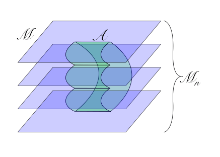
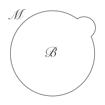
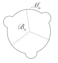
We’ve illustrated the ${n}$ -fold cover below for ${n=4}$ . Each blue sheet represents a copy of the original boundary manifold ${\mathcal{M}}$ , which we’ve glued together along the cuts ${A}$ as follows: in the original Euclidean path integral, we had ${\tau\sim\tau+2\pi}$ at each of the two boundary points of ${A}$ . Now, going to ${2\pi}$ takes us to the second copy, ${4\pi}$ to the third, ${6\pi}$ to the fourth, and finally ${8\pi}$ back to the first; that is, ${\mathcal{M}_n}$ has a ${Z_n}$ symmetry that takes ${\tau\sim\tau+2\pi n}$ .

n-fold_cover

The density matrix is defined via the usual Euclidean path integral:

$\displaystyle \rho=\frac{1}{Z}\int\mathcal{D}\phi e^{-S_E}~,\;\;\;Z=e^{-\beta \hat H}~, \ \ \ \ \ (3)$

where ${S_E}$ is the Euclidean action on ${\mathcal{M}}$ and ${Z}$ is the thermal partition function at inverse temperature ${\beta}$ , with time-evolution operator ${\hat H}$ . Taking ${n}$ copies and computing the trace (i.e., integrating over the fields, with the aforementioned boundary conditions) then yields

$\displaystyle \mathrm{tr}{\rho^n}=\frac{Z_n}{Z^n}~, \ \ \ \ \ (4)$

where we’ve denoted the partition function on the ${n}$ -fold cover by ${Z_n}$ , and the denominator ensures that the normalization is preserved. Substituting this into the above formula for the Rényi entropy, we have

$\displaystyle S_n=\frac{1}{1-n}\left(\ln Z_n-n\ln Z\right), \ \ \ \ \ (5)$

which will prove more tractable in the manipulations to come.

So far we’ve dealt only with the boundary. Now we wish to move into the bulk. To do so requires finding the bulk solution whose boundary is ${\mathcal{M}_n}$ . In general, there may be multiple such solutions; we’ll proceed with the dominant saddle point ${B_n}$ . We then move into the bulk through the differentiate dictionary, which equates the bulk (that is, the on-shell bulk action at large ${N}$ ) and boundary partition functions. Expanding the partition function on ${\mathcal{M}_n}$ in the saddle-point approximation, we therefore have

$\displaystyle Z_n\equiv Z[\mathcal{M}_n]=e^{-S[B_n]+\ldots} \ \ \ \ \ (6)$

where the ellipsis denotes both subleading saddles and ${1/N}$ corrections; we’ll drop these henceforth.

At this point we must address a subtlety lurking in the above, namely: all this ${n}$ -fold cover business assumes ${n\in\mathbb{Z}_+}$ , and hence the ${n\rightarrow1}$ limit obviously requires that we analytically continue to ${n\in\mathbb{R}}$ . But for non-integer ${n}$ , ${Z_n}$ can generally not be written as a partition function with a local action. The reason is that for integer ${n}$ , the fixed points on the boundary of the orbifold ${\mathcal{M}_n/Z_n}$ are simply ${\partial A}$ , from which we can extend ${Z_n}$ locally into the bulk as usual; but for non-integer ${n}$ , we have no regular orbifold structure.

There are two options for proceeding. One is to first calculate ${Z_n}$ for integer values and attempt to analytically continue the result, but this is generally hard. An easier alternative — and the key to the LM derivation — is to do the analytic continuation in the bulk instead. This relies on the observation that ${\mathcal{M}_n}$ has a ${Z_n}$ symmetry that cyclically permutes the ${n}$ replicas, and the assumption that this symmetry extends into the bulk to the dominant saddle ${B_n}$ . In other words, rather than considering the boundary orbifold ${\mathcal{M}_n/Z_n}$ , we instead consider the bulk orbifold ${B_n/Z_n\equiv\hat{B}_n}$ , which is regular everywhere except at the fixed points of the ${Z_n}$ symmetry.

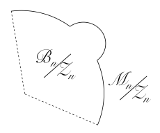
It is important to note that ${\hat{B}_n\neq B_1\equiv B}$ . This can be seen in the illustration below. The left-most image is the original geometry, with a “bump” for illustration. In the middle image, we’ve cut the boundary ${\mathcal{M}}$ , made ${n=3}$ copies, and glued them together to form the ${n}$ -fold cover ${\mathcal{M}_n}$ , with bulk dual ${B_n}$ . The dotted lines illustrate the ${Z_n}$ symmetry, by which we orbifold to create the right-most image. Now one can see that although the boundary orbifold is simply the original manifold (the endpoints are identified), the same is not true in the bulk due to the conical defect. Imagine folding a piece of paper into a cone; away from the tip, it’s still locally flat, but one can detect the presence of the conical singularity by performing a parallel transport around the axis of symmetry. In this sense, the conical defect has a global effect on the geometry, and this is what prevents us from identifying ${B_n/Z_n\equiv\hat B_n}$ with ${B}$ .

orbifold1 orbifold2 orbifold3

These fixed points form a codimension 2 surface with a conical deficit of ${2\pi-2\pi/n}$ ; we shall denote this surface ${C_n}$ . As mentioned above, the fixed points on the boundary orbifold are simply ${\partial A}$ , so this is where ${C_n}$ is anchored on the boundary. (Note that the surface ${C_n}$ is the analogue of the ${U(1)}$ fixed point in the original Gibbons-Hawking analysis).

Before continuing, let’s pause to observe why this procedure allows us to circumvent the restriction on naïve analytic continuation mentioned above, namely that we could not express ${Z_n}$ in terms of a local action. The boundary of ${\hat{B}_n}$ is the boundary orbifold ${\mathcal{M}_n/Z_n}$ , which is simply the original manifold ${\mathcal{M}}$ , with fixed points given by the boundary of the region ${A}$ . The ${Z_n}$ symmetry therefore acts on the boundary of ${\hat{B}_n}$ as ${\tau\rightarrow\tau+2\pi}$ , where ${\tau}$ is the angular coordinate around ${\partial A}$ (that is, ${\tau}$ is simply the thermal time in the Euclidean path integral, which is of course periodic), and there is no obstruction to locally extending the ${\tau}$ coordinate into the bulk such that the ${Z_n}$ symmetry acts on ${\hat{B}_n}$ in the same way. The fixed points of the action of ${Z_n}$ on ${\hat{B}_n}$ give us ${C_n}$ as described above. The key is that, since we can locally extend the symmetry from the boundary of the original manifold, it’s no longer necessary to think of ${C_n}$ as the ${Z_n}$ orbifold of some regular geometry, and thus we’re free to analytically continue away from integer ${n}$ .

The upshot of all this is that the ${Z_n}$ symmetry allows us to write

$\displaystyle S\left[B_n\right]=nS[\hat{B}_n]~, \ \ \ \ \ (7)$

simply because, by extending the ${Z_n}$ symmetry in the above manner, we’re guaranteed that the contribution from the dominant saddle point of the ${n}$ -fold cover, ${S\left[B_n\right]}$ , is simply ${n}$ times that from the orbifold, ${S[\hat{B}_n]}$ . This expression is useful because, in conjunction with the above expression for the partition function (dropping the higher order terms), we may write the Rényi entropy as

$\displaystyle S_n=\frac{n}{n-1}\left( S[\hat{B}_n]-S[B]\right) \ \ \ \ \ (8)$

where ${B\equiv \hat{B}_1}$ is simply the original bulk dual of ${A}$ .

It now remains to analytically continue ${\hat{B}_n}$ to non-integer ${n}$ , so that we can take the ${n\rightarrow1}$ limit of this expression. In the process, we shall see that ${C_n}$ is precisely the minimal bulk surface associated with the original region ${A\subset\mathcal{M}}$ , which therefore enables us to prove RT. There are a couple ways to find the analytic continuation of ${\hat{B}_n}$ , but here we will follow the so-called squashed cone method.

To begin, we choose a set of local coordinates such that ${\rho}$ parametrizes the radial (minimal) distance to ${C_n}$ from the boundary, with angular coordinate ${\tau}$ :

$\displaystyle \mathrm{d} s^2=\rho^{-2\epsilon}\left(\mathrm{d}\rho^2+\rho^2\mathrm{d} \tau^2\right)+\left( g_{ij}+2K_{aij}x^a\right)\mathrm{d} y^i\mathrm{d} y^j+\ldots \ \ \ \ \ (9)$

where ${a,b,\ldots}$ are indices in the ${\left(\rho,\tau\right)}$ plane orthogonal to ${C_n}$ , while ${i,j,\ldots}$ are indices along ${C_n}$ . ${K_{aij}}$ is the extrinsic curvature tensor of ${C_n}$ . The ellipsis denotes terms higher order in ${\rho}$ , which are subleading near ${C_n}$ (since ${\rho\rightarrow0}$ there). This is called the squashed cone because the first term resembles the line element in polar coordinates (the “cone”; recall the familiar Euclidean black hole geometry), but the second term, with the index ${a}$ running over ${\tau}$ , breaks the U(1) symmetry (the “squashed”).

In these coordinates, one sees that the conical deficit at ${\rho=0}$ is ${2\pi\epsilon}$ as follows: rewriting the metric in terms of the proper distance ${r}$ , we have

$\displaystyle \rho^{-\epsilon}\mathrm{d}\rho=\mathrm{d} r\implies \frac{\rho^{1-\epsilon}}{1-\epsilon}=r\implies \mathrm{d} s^2=\mathrm{d} r^2+r^2(1-\epsilon)^2\mathrm{d}\tau^2+\ldots \ \ \ \ \ (10)$

hence we must identify

$\displaystyle \tau\sim\tau+\frac{2\pi}{1-\epsilon} \ \ \ \ \ (11)$

and thus, Taylor expanding around ${\epsilon=1}$ , the deficit angle is

$\displaystyle 2\pi\left(1-\frac{1}{1-\epsilon}\right)= 2\pi\epsilon+O\left(\epsilon^2\right)~. \ \ \ \ \ (12)$

However, we know from the general considerations above that the deficit angle must be ${2\pi-2\pi/n}$ for ${n\in\mathbb{Z}}$ , and therefore (to leading order) we must have ${\epsilon=1-1/n}$ .

To find ${\hat{B}_n}$ , one solves the bulk equations of motion with the unconventional IR boundary condition that the metric should resemble the form above near ${C_n}$ . (The boundary condition is “unconventional” because we normally impose a UV boundary condition as per AdS/CFT; in this case however, the boundary of ${\hat{B}_n}$ is of course ${\mathcal{M}}$ ). In the course of doing so, one finds that, in complex coordinates ${z\equiv\rho e^{i\tau}}$ , the ${zz}$ -component of the Einstein equation is

$\displaystyle R_{zz}=2K_z\frac{\epsilon}{z}+\ldots~, \ \ \ \ \ (13)$

where ${K_z=K_{zij}g^{ij}}$ is the trace of the extrinsic curvature. The first term is clearly divergent as ${\rho\rightarrow0}$ , while the remaining terms are higher-order in ${\epsilon}$ (and hence less divergent in this limit).

Now, the stress tensor from the matter (i.e., bulk) sector should be finite—it’s regular at integer ${n}$ because ${B_n}$ is regular, and as per our discussion above, this well-behavedness should be preserved under ${Z_n}$ . Hence, since the l.h.s. is finite, the ${1/z}$ divergence on the r.h.s. must vanish. This implies that we must have

$\displaystyle K_z=0 \ \ \ \ \ (14)$

in the ${n\rightarrow1}$ limit. But this is precisely the condition for a minimal surface! And since this condition is satisfied when ${\rho=0}$ , we conclude that ${C_n}$ is indeed the minimal surface associated to the boundary region ${A}$ .

We now have all the ingredients in place to prove RT, but we must perform one final computation. Upon taking the ${n\rightarrow1}$ limit of ${S_n}$ , we have

$\displaystyle \begin{aligned} \lim_{n\rightarrow1}S_n&=\lim_{n\rightarrow1}\frac{n}{n-1}\left( S[\hat{B}_n]-S[B]\right)\\ &=\left[S[\hat{B}_n]-S[B]+n\left(\partial_nS[\hat{B}_n]-\partial_nS[B]\right)\right]\bigg|_{n=1}\\ &=\partial_nS[\hat{B}_n]\bigg|_{n=1}=S~, \end{aligned} \ \ \ \ \ (15)$

and thus we must calculate the variation of the action to leading order in ${(n-1)}$ . (In going to the second line, l’Hospital’s rule is justified since ${\hat B_1=B_1\equiv B}$ ). This will introduce boundary terms, which — as in the aforementioned Gibbons-Hawking result — turn out to be all-important.

We will not compute these boundary terms explicitly here; one can find the analysis in the LM paper. Rather, we will present the following simple heuristic argument offered by Dong. At ${n=1}$ there is no conical defect, and therefore the only contribution must be from boundary terms in the action. Since ${C_1}$ is non-singular, it gives no contribution, and hence we should excise a small region around ${C_1}$ , thereby introducing a boundary which is precisely the area of ${C_1}$ . Thus,

$\displaystyle S\sim\mathrm{Area\left( C_1\right)}~, \ \ \ \ \ (16)$

where, of course, fixing the constant of proportionality requires performing the explicit computation. Upon fixing this, and using the above fact that ${C_1}$ is precisely the minimal surface associated to the region ${A}$ , one indeed obtains RT.

If the above argument about excising ${C_1}$ seems sketchy, consider again the expression ${S[B_n]=nS[\hat B_n]}$ . The l.h.s. is the bulk dual of the entire ${n}$ -fold cover ${\mathcal{M}_n}$ , and is therefore regular everywhere; in particular, it has no conical deficit. Thus, if we want this expression to hold, the r.h.s. cannot include any contribution from ${C_n}$ either.

1 Response to Generalized gravitational entropy

Pingback: Islands behind the horizon | Ro's blog