Quantum 101

Reference: John Preskill’s notes on Quantum Information and Computation.

In quantum mechanics, a state is a complete description of a physical system. Mathematically, it is given by a ray (an equivalence class of vectors) in Hilbert space, ${\mathcal{H}}$ , which is a vector space endowed with an inner product, and which is complete with respect to the norm induced by the latter. Simply put, Hilbert space is the abstract vector space in which quantum states “live”.

Hilbert spaces can be real or complex, finite- or infinite-dimensional; for definiteness we’ll assume complex, finite-dimensional Hilbert spaces here. The inner product is simply a map that associates an element of the field to pairs of elements in the vector space; in this case, ${\left<\cdot,\cdot\right>:\mathcal{H}\times\mathcal{H}\rightarrow\mathbb{C}}$ . In Dirac’s bra-ket notation, vectors (states) in ${\mathcal{H}}$ are denoted ${\left|\psi\right>}$ , and dual vectors (operators, which act as linear functionals on the states) are denoted ${\left<\psi\right|}$ . The properties of the inner product ${\left<x,y\right>\equiv\left<y|x\right>}$ may then be written as follows:

Positivity: ${\left<\psi|\psi\right>\geq0}$ , with equality iff ${\left|\psi\right>=0}$ .
Linearity: ${\left<\phi\right|\left( a\left|\psi_1\right>+b\left|\psi_2\right>\right)=a\left<\phi|\psi_1\right>+b\left<\phi|\psi_2\right>}$ .
Skew symmetry: ${\left<\phi|\psi\right>=\left<\psi|\phi\right>^*}$ .

The inner product induces a norm, ${||\psi||=\left<\psi|\psi\right>^{1/2}}$ , which defines the distance between states in ${\mathcal{H}}$ . Any inner product space with such a distance function is a metric space, also known as a pre-Hilbert space. The aforementioned completeness criterion is what elevates a pre-Hilbert space to a Hilbert space: a pre-Hilbert space is complete if every Cauchy sequence converges with respect to the norm to an element in the space (intuitively, there are no “missing points”). The completeness criterion is important for infinite-dimensional Hilbert spaces, where it ensures the convergence of eigenfunction expansions that one encounters in, e.g., Fourier analysis.

Note that we are free to choose the normalization ${\left<\psi|\psi\right>=1}$ , since this merely amounts to choosing a representative of the equivalence class of vectors that differ by a nonzero complex scalar. In this sense, both ${\left|\psi\right>}$ and ${e^{i\alpha}\left|\psi\right>}$ represent the same state; only relative phase changes between states in a superposition are physically meaningful.

Although states are the basic mathematical objects in this formalism, we never measure them. Rather, we measure observables, which are self-adjoint (a.k.a. Hermitian) operators that act as linear maps on states, ${A:\mathcal{H}\rightarrow\mathcal{H}}$ . Such an operator has a spectral representation, meaning that its eigenstates form a complete orthonormal basis in ${\mathcal{H}}$ . This allows us to write an observable ${A}$ as

$\displaystyle A=\sum_n a_n P_n~, \ \ \ \ \ (1)$

where ${P_n}$ is the orthogonal projection onto the space of eigenvectors with eigenvalue ${a_n}$ (such orthogonal projections can be proven to exist for complete inner product spaces, e.g., ${\mathcal{H}}$ ). In the simple case where ${a_n}$ is non-degenerate, ${P_n}$ is the projection onto the corresponding eigenvector, ${P_n=\left|n\right>\left<n\right|}$ . Of course, given the unit normalization above, the projection operators satisfy ${P_nP_m=\delta_{mn}P_n}$ and ${P_n^\dagger=P_n}$ . (Note that the spectral theorem is more subtle for unbounded operators in infinite-dimensional spaces, but that will not concern us here).

The numerical result of a measurement in quantum mechanics is given by the eigenvalue of the observable in question, ${A}$ . This implies that the system must, at the instant of measurement, be in an eigenstate of ${A}$ with the measured eigenvalue. If the quantum state immediately prior to a measurement is ${\left|\psi\right>}$ , then the outcome ${a_n}$ is obtained with probability

$\displaystyle \mathrm{Prob}\left( a_n\right)=||P_n\left|\psi\right>||^2=\left<\psi|P_n\right>~, \ \ \ \ \ (2)$

and the normalized quantum state with eigenvalue ${a_n}$ is therefore

$\displaystyle \frac{P_n\left|\psi\right>}{\left<\psi|P_n\right>^{1/2}}~. \ \ \ \ \ (3)$

This is the point at which probability notoriously enters the picture; we’ll have more to say about this later. Note that, since the system is now in an eigenstate, immediately repeating the measurement will yield the same eigenvalue with probability 1.

The fact that the measurement process appears to induce such decisiveness on the part of the state leads to the notion of “wave function collapse”, which is a horribly misleading oversimplification to which we will return. Suffice to say that wave functions don’t collapse, but we’ve a bit more math to cover before the reality can be made precise.

So much for states and observables. What about dynamics? As in classical mechanics, the Hamiltonian ${H}$ is the generator of time translations, and its expectation value gives the energy of the state. The latter is a measurable quantity, which implies that in order to be a well-defined physical observable, the Hamiltonian operator must be self-adjoint, ${H^\dagger=H}$ . By Stone’s theorem, the exponential of a self-adjoint operator is unitary; thus if ${U=e^{-iHt}}$ , then ${U}$ is a bounded linear operator on ${\mathcal{H}}$ that satisfies ${U^\dagger U=1}$ . Mathematically, this is why time evolution in quantum mechanics is unitary. Physically, this is simply the statement that time evolution preserves the inner product; i.e., that probabilities continue to sum to 1 (since, under time-evolution by a Hermitian operator ${U}$ , ${\left<x|y\right>\rightarrow\left<x|U^\dagger U|y\right>=\left<x|y\right>}$ ). Note that here we’re implicitly assuming that ${H}$ is time-independent, in order to write the time translation operator as the exponential thereof. For time-dependent cases, one can still show ${H^\dagger=H}$ perturbatively in ${t}$ , it’s just less elegant.

Given such an operator ${U}$ , the evolution of a state over some finite interval ${t}$ is unitary, and may be written

$\displaystyle \left|\psi(t)\right>=U(t)\left|\psi(0)\right>=e^{-iHt}\left|\psi(0)\right>~, \ \ \ \ \ (4)$

where in the second equality we’ve assumed ${H}$ to be time-independent. If we then consider an infinitesimal transformation ${\delta t}$ and expand both the left- and right-hand sides to first order, we have

$\displaystyle \left|\psi(\delta t)\right>=\left|\psi(0)\right>+\delta t\frac{\mathrm{d}}{\mathrm{d} t}\left|\psi(0)\right>=\left(1-iH\delta t\right)\left|\psi(0)\right>~. \ \ \ \ \ (5)$

Comparing terms at linear order, we recognize the Schrödinger equation,

$\displaystyle \frac{\mathrm{d}}{\mathrm{d} t}\left|\psi(t)\right>=-iH\left|\psi(t)\right>~, \ \ \ \ \ (6)$

which describes the evolution of states in the Schrödinger picture, wherein states are time-dependent while operators (including observables) are constants. This is precisely the opposite of the Heisenberg picture, wherein operators carry the time-dependence while states are constant. The two pictures are related by a change of basis, analagous to the relation between active and passive transformations. A third picture, the interaction picture, is often later introduced as a rather ham-fisted compromise between these two; it forms a fantastically successful premise for perturbation theory, but it doesn’t actually exist (see Haag’s theorem).

Note that unitary evolution, as encapsulated in the Schrödinger equation, is entirely deterministic: specification of an initial state ${\left|\psi(t)\right>}$ allows us to predict the state at any future time. But as described above, measurement is probabilistic: despite our infinite ability to predict future states, we cannot make definite predictions about measurement outcomes. One of the deepest (and most controversial) aspects of quantum mechanics is how deterministic evolution can nonetheless lead to probabilistic outcomes. Preskill quite aptly refers to this juxtaposition as a “disconcerting dualism”, and we shall return to it below.

Another interesting observation is that according to the Schrödinger equation, quantum mechanical evolution is linear, in contrast to the non-linear evolution often encountered in classical theories. This is tied up with the issue of probability above: probability theory is fundamentally linear. But the connection isn’t quite so straightforward.

As an aside, the linearity of quantum mechanics is why quantum chaos is so subtle. Naïvely, quantum systems should be incapable of supporting chaos, since small perturbations to the initial state don’t wildly change the evolution in the case of linear dynamics. However, two states which are close in Hilbert space can nonetheless yield wildly different measurements. Quantum chaos has important implications in a number of areas, particularly holography and black holes; but that’s a subject for another post.

So, to summarize, we’ve seen that in quantum mechanics, states are vectors in Hilbert space, observables are Hermitian operators, symmetries are unitary operators, and measurements are orthogonal projections.

Now here’s the kicker: everything we’ve said so far applies only to a single, isolated system. This is an idealization that simply does not exist. Another way to phrase this is that the formulation above only holds if applied to the entire universe. Even ignoring the issue of how one would make a measurement in such a scenario, this is clearly not a realistic description. In fact, it’s frankly wrong: in general (that is, when considering subsystems) states are not rays, measurements are not orthogonal projections, and evolution is not unitary!

The simplest extension of the above is to consider a bipartite system, the Hilbert space for which is a tensor product of the Hilbert spaces of the constituents, ${\mathcal{H}=\mathcal{H}_A\otimes\mathcal{H}_B}$ . Given an orthonormal basis ${\{\left|i\right>_A\}}$ for ${\mathcal{H}_A}$ and ${\{\left|j\right>_B\}}$ for ${\mathcal{H}_B}$ , an arbitrary pure state of ${\mathcal{H}_A\otimes\mathcal{H}_B}$ can be expanded as

$\displaystyle \left|\psi\right>_{AB}=\sum_{i,j}a_{ij}\left|i\right>_A\otimes\left|j\right>_B~, \ \ \ \ \ (7)$

where, by unitarity, the eigenvalues satisfy ${\sum_{i,j}|a_{ij}|^2=1}$ . We’ve referred to this as a pure state in contrast to a mixed state; the former correspond to rays in the total Hilbert space, while the latter do not. This is the first crucial correction alluded to above.

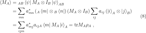
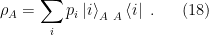
Let us now consider an observable that acts only on subsystem ${A}$ , ${M_A\otimes I_B}$ . Its expectation value is

$\displaystyle \begin{aligned} \left<M_A\right>&={}_{AB}\left<\psi\right|M_A\otimes I_B\left|\psi\right>_{AB}\\ &=\sum_{mn}a_{mn}^*\left({}_A\left<m\right|\otimes{}_B\left<n\right|\right)\left( M_A\otimes I_B\right)\sum_{ij}a_{ij}\left(\left|i\right>_A\otimes\left|j\right>_B\right)\\ &=\sum_{ijm}a_{mj}^*a_{ij}{}_A\left<m\right| M_A\left|i\right>_A =\mathrm{tr}{M_A\rho_A}~, \end{aligned} \ \ \ \ \ (8)$

where we’ve introduced the reduced density matrix

$\displaystyle \rho_A=\mathrm{tr}_B\left(\left|\psi\right>_{AB~AB}\left<\psi\right|\right)~. \ \ \ \ \ (9)$

In contrast to the trace, which is a scalar-valued function given by the sum of eigenvalues, the partial trace w.r.t. ${B}$ is an operator-valued function given by summing over the basis elements of ${B}$ :

$\displaystyle \mathrm{tr}_B\left(\left|\psi\right>_{AB~AB}\left<\psi\right|\right) =\sum_j\big._B\left<j|\psi\right>_{AB~AB}\left<\psi|j\right>_B =\sum_{ijm}a_{mj}^*a_{ij}\left|i\right>_{A~A}\left<m\right|~. \ \ \ \ \ (10)$

The elegant expression for the expectation value ${\left<M_A\right>}$ above then follows by the cyclic property of the trace.

The reduced density matrix will play a central role in what follows, so it’s worth elaborating the properties that follow from the definition above (in particular the explicit form (10)):

Hermiticity: ${\rho_A=\rho_A^\dagger}$ .
Non-negativity (of its eigenvalues): ${\forall~\left|\psi\right>_A}$ , ${\big._A\left<\psi\right|\rho_A\left|\psi\right>_A=\sum_j\big|\sum_ia_{ij}\big._A\left<\psi|i\right>_A\big|^2\ge0}$ .
Unit norm: ${\mathrm{tr}{\rho_A}=\sum_{ij}|a_{ij}|^2=1}$ (since ${\left|\psi\right>_{AB}}$ is normalized).

As mentioned above, pure states are rays in Hilbert space, but mixed states are not. However, both are described by a reduced density matrix, which therefore provides a suitably general definition of quantum states. In the case of a pure state, 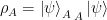${\rho_A=\left|\psi\right>_A\big._A\left|\psi\right>}$ , which is the projection operator onto the state (that is, onto the one-dimensional space spanned by ${\left|\psi\right>_A}$ ). The density matrix for a pure state is therefore idempotent, ${\rho^2=\rho}$ . In contrast, for a general (mixed) state in the diagonal basis ${\{\left|\psi_a\right>\}}$ ,

$\displaystyle \rho_A=\sum_ap_a\left|\psi_a\right>\left<\psi_a\right|~, \ \ \ \ \ (11)$

where the eigenvalues satisfy ${0<p_a\le1}$ and ${\sum_ap_a=1}$ . It follows that a pure state has only a single non-zero eigenvalue, which must be 1, while a mixed state contains two or more terms in the sum (and ${\rho^2\neq\rho}$ ).

As alluded above, in a coherent superposition of states, the relative phase is physically meaningful (i.e., observable). This is merely a consequence of the linearity of the Schrödinger equation: any linear combination of solutions is also a solution. In contrast, the mixed state ${\rho_A}$ is an incoherent superposition of eigenstates ${\{\left|\psi_a\right>\}}$ , meaning that the relative phases are experimentally unobservable. This gives rise to the concept of entanglement: when two systems ${A}$ and ${B}$ interact, they become entangled (i.e., correlated). This destroys the coherence of the original states such that some of the phases in the superposition become inaccessible if we measure ${A}$ alone. Henceforth we will reserve the unqualified “superposition” to refer to the former case.

We should note that probability again enters this updated picture when we consider that the expectation value of any observable ${M}$ acting on the subsystem described by ${\rho}$ is

$\displaystyle \left<M\right>=\mathrm{tr}{M\rho}=\sum_ap_a\left<\psi_a|M\right>~, \ \ \ \ \ (12)$

which leads to the interpretation of ${\rho}$ as describing a statistical ensemble of pure states ${\left|\phi_a\right>,}$ each of which occurs with probability ${p_a}$ . But we’re not quite ready to address the associated interpretive questions just yet.

As a concrete example, consider the spin state

$\displaystyle \left|\uparrow_x\right>=\frac{1}{\sqrt{2}}\left(\left|\uparrow_z\right>+\left|\downarrow_z\right>\right)~, \ \ \ \ \ (13)$

which is a (coherent) superposition of spins along the ${z}$ -axis. Measuring the spin along the x-axis will result in ${\left|\uparrow_z\right>}$ or ${\left|\downarrow_z\right>}$ with probability ${\frac{1}{2}}$ each; e.g., from (2):

$\displaystyle \mathrm{Prob}\left(\uparrow_z\right)=||P_{\uparrow_z}\left|\uparrow_x\right>||^2 =\frac{1}{2}\left(\left<\uparrow_z|\uparrow_z\right>\right)^2=\frac{1}{2}~. \ \ \ \ \ (14)$

In contrast, the ensemble in which each of these states occurs with this probability is

$\displaystyle \rho=\frac{1}{2}\left(\left|\uparrow_z\right>\left<\uparrow_z\right|+\left|\downarrow_z\right>\left<\downarrow_z\right|\right)=\frac{1}{2}I~. \ \ \ \ \ (15)$

But since the identity is invariant under a unitary change of basis ( ${U^\dagger IU=I}$ ), we can obtain the state along an arbitrary axis ${\left|\psi(\theta,\phi)\right>}$ by applying a suitable unitary transformation to ${\left|\uparrow_z\right>}$ without changing the right-hand side. As a consequence, measuring the spin along any axis yields a completely random result:

$\displaystyle \mathrm{tr}{\left|\psi(\theta,\phi)\right>\left<\psi(\theta,\phi)\right|\rho}=\frac{1}{2}~. \ \ \ \ \ (16)$

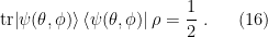
In other words, we obtain spin up or down with equal probability, regardless of what we do. This is a reflection of the fact that the relative phases in a superposition are observable, but those in an ensemble are not. A mixed state can thus be thought of as an ensemble of pure states in many different ways, all of which are experimentally indistinguishable. (As an aside, further clarity on these relationships can be gained by studying the Bloch sphere, which I shall not digress upon here).

A bipartite pure state can be expressed in a standard form, which is often very useful. One begins by observing that an arbitrary state ${\left|\psi\right>_{AB}\in\mathcal{H}_A\otimes\mathcal{H}_B}$ may be expanded as

$\displaystyle \left|\psi\right>_{AB}=\sum_{i,j}a_{ij}\left|i\right>_A\left|j\right>_B=\sum_i\left|i\right>_A\left|\tilde i\right>_B~, \ \ \ \ \ (17)$

where ${\{\left|i\right>_A\}}$ and ${\{\left|j\right>_B\}}$ are the orthonormal bases defined in (7), and in the second equality we’ve defined a new basis ${\left|\tilde i\right>_B=\sum_ja_{ij}\left|j\right>_B}$ . A priori, ${\{\left|\tilde i\right>_B\}}$ need not be orthonormal. However, since ${\{\left|i\right>_A\}}$ is, we are free to choose it such that ${\rho_A}$ is diagonal (cf. (11)), in which case we can write the reduced density matrix that describes subsystem ${A}$ alone as

$\displaystyle \rho_A=\sum_ip_i\left|i\right>_{A~A}\left<i\right|~. \ \ \ \ \ (18)$

However, by definition (9), this is also equivalent to tracing out system ${B}$ ,

$\displaystyle \begin{aligned} \rho_A&=\mathrm{tr}_B\left(\left|\psi\right>_{AB~AB}\left<\psi\right|\right) =\mathrm{tr}_B\left(\sum_{ij}\left|i\right>_A\left|\tilde i\right>_{B~A}\left<j\right|\big._{B}\left<\tilde j\right|\right)\\ &=\sum_{ij}\left|i\right>_{A~A}\left<j\right|\sum_k\big._B\left<\tilde j|k\right>_B\big._B\left<k|\tilde i\right>_B =\sum_{ij}\big._B\left<\tilde j|\tilde i\right>_B\left|i\right>_{A~A}\left<j\right|~. \end{aligned} \ \ \ \ \ (19)$

And therefore, it must be the case that

$\displaystyle \big._B\left<\tilde j|\tilde i\right>_B=\delta_{ij}p_i \ \ \ \ \ (20)$

i.e., the new basis 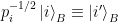${\{\left|\tilde i\right>_B\}}$ is orthogonal after all! Furthermore, by simply rescaling the vectors by ${p_i^{-1/2}\left|i\right>_B\equiv\left|i'\right>_B}$ , we find that we can express the bipartite state (17) as

$\displaystyle \left|\psi\right>_{AB}=\sum_i\sqrt{p_i}\left|i\right>_A\left|j\right>_B=\sum_i\left|i\right>_A\left|\tilde i\right>_B~, \ \ \ \ \ (21)$

which is the Schmidt decomposition of the bipartite pure state ${\left|\psi\right>_{AB}}$ in terms of a particular orthonormal basis of ${\mathcal{H}_A\otimes\mathcal{H}_B}$ . Note that our derivation was completely general; any bipartite pure state can be expressed in this form, though of course the particular orthonormal basis employed will depend on the state (that is, we can’t simultaneously expand ${\left|\psi\right>_{AB}}$ and ${\left|\phi\right>_{AB}}$ using the same orthonormal basis for ${\mathcal{H}_A\otimes\mathcal{H}_B}$ ).

Observe that by tracing over one of the Hilbert spaces in (21), we find that both ${\rho_A}$ and ${\rho_B}$ have the same nonzero eigenvalues, e.g.,

$\displaystyle \rho_B=\mathrm{tr}_A\left(\left|\psi\right>_{AB~AB}{\left<\psi\right|}\right)=\sum_ip_i\left|i'\right>_B\big._B\left<i'\right|~, \ \ \ \ \ (22)$

though since the dimensions of ${\mathcal{H}_A}$ and ${\mathcal{H}_B}$ need not necessarily be equal, the number of zero eigenvalues can still differ. The fact that ${\rho_A}$ and ${\rho_B}$ have no degenerate non-zero eigenvalues implies that they uniquely determine the Schmidt decomposition: one can diagonalize the reduced density matrices, and then pair up eigenstates with the same eigenvalue to determine (21). (There is still the potential for ambiguity in the basis if either ${\rho_A}$ or ${\rho_B}$ individually has degenerate eigenvalues—to wit, which ${\left|i'\right>_B}$ gets paired with which ${\left|i\right>_A}$ ).

The Schmidt decomposition is useful for characterizing whether pure states are separable or entangled (for mixed states, the situation is more subtle). In particular, the bipartite pure state above, ${\left|\psi\right>_{AB}}$ is separable iff there is only one non-zero Schmidt coefficient ${p_i}$ . Otherwise, the state is entangled. If all the Schmidt coefficients are equal (and non-zero), then the state is maximally entangled. On account of this classification, it is common to associated a Schmidt number to the state ${\left|\psi\right>_{AB}}$ , which is the number of non-zero eigenvalues (equivalently, the number of terms) in the decomposition (note that this implies the Schmidt number is a positive integer). Thus a pure state is separable iff its Schmidt number is 1. In this case we can write it as a direct product of states in ${\mathcal{H}_A}$ and ${\mathcal{H}_B:}$ ${\left|\psi\right>_{AB}=\left|\phi\right>_A\otimes\left|\chi\right>_B}$ , which further implies that ${\rho_A=\left|\phi\right>_A\big._A\left<\phi\right|}$ and ${\rho_B=\left|\chi\right>_B\big._B\left<\chi\right|}$ are each pure. In contrast, an entangled state, with Schmidt number greater than 1, has no such direct product expression, in which case ${\rho_A}$ and ${\rho_B}$ are mixed.

Entanglement is quantified by the von Neumann entropy. Entanglement entropy is a tremendously rich topic in itself, to say nothing of its connections to other areas of physics, and thus we defer further discussion elsewhere.

To summarize, it is only in the case for idealized, isolated systems (i.e., the entire universe) that quantum states may be described by rays in Hilbert space. In reality, since we always deal with subsystems, states are given by (reduced) density matrices defined by tracing out the complement of the Hilbert space under consideration. (The Hilbert spaces themselves are associated with spatial regions, and thus what we mean is that we trace over all degrees of freedom localized in the complement of our subregion. As mentioned elsewhere however, this is generally still too naïve).

It remains to justify our earlier claim that generic measurements are not orthogonal projections, and evolution non-unitary. In the course of doing so, we shall resolve Preskill’s “disconcerting dualism” between determinism and probability, and explain why the notion of wave-function collapse is an illusion. But this will require us to develop slightly beyond the basic mathematical machinery above, and as such we partition the discussion into Part 2.

Quantum 101

Leave a Reply Cancel reply

Archives

Meta

Follow me!

Legal stuff

Quantum 101

Share this:

Like this:

Leave a Reply Cancel reply

Archives

Meta

Follow me!

Legal stuff