I was recently** asked to give a lecture on black hole thermodynamics and the associated quantum puzzles, which provided a perfect excuse to spend some time reviewing one of my favourite subjects: quantum field theory (QFT) in curved spacetime. I’ll mostly follow the canonical reference by Birrell and Davies [1], and will use this series of posts to highlight a number of important and/or interesting aspects along the way. I spent many a happy hour with this book as a graduate student, and warmly recommend it to anyone desiring a more complete treatment.

**(That is, “recently” when I started this back in February. I had intended to finish the series before posting the individual parts, to avoid retroactive edits as my understanding and plans for future segments evolves, but alas the constant pressure to publish (or, perhaps more charitably, the fact that I don’t get paid to teach a course on this stuff) means that studies of this sort are frequently pushed down my priority list (and that was before an international move in the midst of a global pandemic, for those wondering why I haven’t posted in so long). Since such time constraints are likely to continue — on top of which, I have no fixed end-point in mind for this vast subject — I’ve decided to release the first few parts I’ve been sitting on, lest they never see the light of day. I hope to add more installments as time permits.)

I’m going to start by discussing Green functions (commonly but improperly called “Green’s functions”), which manifest one of the deepest relationships between gravity, quantum field theory, and thermodynamics, namely the thermodynamic character of the vacuum state. Specifically, the fact that Green functions are periodic in imaginary time — also known as the KMS or Kubo-Martin-Schwinger condition — hints at an intimate relationship between Euclidean field theory and statistical mechanics, and underlies the thermal nature of horizons (including, but not limited to, those of black holes).

For simplicity, I’ll stick to Green functions of free scalar fields , where the -vector . As a notational aside, I will depart from [1] in favour of the modern convention in which the spacetime dimension is denoted , with Greek indices running over the full -dimensional spacetime, and Latin indices restricted to the -dimensional spatial component. While I’m at it, I should also warn you that [1] uses the exceedingly unpalatable mostly-minus convention , whereas I’m going to use mostly-plus . The former seems to be preferred by particle physicists, because they share with small children a preference for timelike 4-vectors to have positive magnitude. But the latter is generally preferred by relativists and most workers in high-energy theory and quantum gravity, because 3-vectors have no minus signs (i.e., it’s consistent with the non-relativistic case, whereas mostly-plus yields a negative-definite metric), raising and lowering indices involves flipping only a single sign (arguably the most important for our purposes, since we’ll be Wick rotating between Lorentzian and Euclidean signature; mostly-plus would again lead to a negative-definite Euclidean metric), and the extension to general dimensions contains only a single in the determinant (as opposed to a factor of in mostly-minus).

Notational disclaimers dispensed with, the Lagrangian density is

where is the Minkowski metric (no curved space just yet). By applying the variational principle to the action

we obtain the familiar Klein-Gordon equation

where . The general solution, upon imposing that be real-valued, is

where (note that [1] restricts to the case of a discrete spectrum, as though the system were in a box; useful for imposing an IR regulator, but unnecessary for our purposes, and potentially problematic if we want to consider Lorentz boosts or Euclidean continuations). Here is the annihilation operator that kills the vacuum state, i.e., (so , by extension, is a real-valued field operator).

One last (lengthy, but important) notational aside: different authors make different choices for the integration measure , which affects a number of later formulas, and can cause confusion when comparing different sources. The convention I’m using is physically well-motivated in that it makes the measure Lorentz invariant while encoding the on-shell condition . That is, the Lorentz invariant measure in the full -dimensional spacetime is . If we then impose the on-shell condition along with (in the form of the Heaviside function ), we have

We now use the following trick: if a smooth function has a root at , then we may write

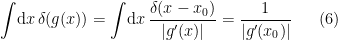
where the prime denotes the derivative with respect to . In the present case, , and (note that the Heaviside function will select the positive root). Thus

Finally, since and are related by a Fourier transform, we must adopt a convention for the associated factor of . Mathematicians seem to prefer splitting this so that both and get a factor of , but physicists favour simply attaching it all to the momentum, so that

which further implies the convention

as one can readily verify by substituting into (or vice versa):

Thus our choice for the measure in (4):

(I realize that was a bit tedious, but setting one’s conventions straight will pay dividends later. Trust me: I’ve lost hours trying to sort out factors of and the like for failure to invest this time at the start).

We can now consider vacuum expectation values of products of field operators . For free scalar fields, these can always be decomposed into two-point functions, which therefore play a defining role. In particular, we can construct various Green functions of the wave operator from the two-point correlator , including the familiar Feynman propagator. Following [1], we’ll denote the expectation values of the commutator and anticommutator as follows:

where on the far right-hand sides are the so-called positive/negative frequency Wightman functions,

Note that while physicists call all of these Green functions, they’re technically kernels, i.e.,

One can immediately verify this by observing that since acts only on (that is, ), it reduces to the Klein-Gordon equation above for the Wightman functions, from which the others follow.

Using these building blocks, we can consider the true Green functions

which is the familiar (time-ordered, ) Feynman propagator, and

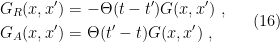
which are the retarded (R) and advanced (A) propagators. All three of these are Green functions of the wave operator, i.e.,

Let’s verify this for the Feynman propagator; the others are similar. Using the fact that , we have

Now observe that by virtue of the delta function, the equal-time commutator means that in the first line, . And since the delta function itself is even, this implies that the first two terms cancel, so we continue with just the second line:

where in the second step, we have used the fact that the delta function is even, and identified the conjugate momentum . Then by (14), the second line will vanish for all values of when we add in the term of the wave operator, and the first line is just (minus) the equal-time commutator . Hence

Thus the Feynman propagator is indeed a Green function of the wave operator ; similarly for and .

The reason I’ve been calling the Green functions “propagators” is that, unlike the kernels , they represent the transition amplitude for a particle (virtual or otherwise) propagating from to , subject to appropriate boundary conditions. To see this, consider the integral representation

where . Due to the poles at 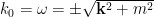, we need to choose a suitable contour for the integral to be well-defined (analytically continuing to ). The particular choice of contour determines which of the kernels or Green functions we obtain. (As for how we obtained (21) in the first place, one can directly substitute in the mode expansion (4) to the definitions, and convert the Heaviside functions into an appropriate integral. An easier way, at least for the Green functions, is to simply Fourier transform the wave equation (17):

Since this expression (i.e., the delta function) is even in , we may absorb the sign into the integration variable, and identify

whereupon Fourier transforming back to position space yields (21). As alluded above however, these expressions don’t make sense without specifying a pole prescription, so this argument isn’t very rigorous; it’s just a quick-and-dirty way of convincing yourself that (21) is plausible.)

To make sense of this expression, we split the integral based on the two poles of :

Now, the boundary conditions of the propagator at hand determines the prescription, i.e., which of the poles we want to enclose with the choice of contour. Consider first the retarded propagator : the boundary condition implicit in (16) is that the function should vanish when (where ). Conversely, when , we must close the contour in the negative half-plane so that , and the integral converges. Thus we should introduce factors of such that both poles are slightly displaced into the lower half-plane. We can then apply Cauchy’s integral formula to correctly capture the poles at , and then take :

where in the penultimate line, we have taken in the second term, using the fact that the integration over all (momentum) space is even; in the last line, we have used the mode expansion (4) and the commutation relation . Note that to yield the correct signs, we’ve chosen the contour to run counter-clockwise (note the factor of ), which means that it runs from to along the real axis. The prescription for the advanced propagator is precisely similar, except we deform both poles in the positive complex direction (so that the integral vanishes when we close the contour below, as required for ), and the non-vanishing contribution comes from closing the contour in the positive half-plane, encircling both poles clockwise rather than counter-clockwise (so that the integral again runs from to along the real axis).

Note that are superpositions of both positive () and negative () energy modes, which is necessary in order for them to vanish outside their prescribed lightcones (past and future, respectively). In contrast, the Heaviside functions in the Feynman propagator are tantamount to imposing boundary conditions such that it picks up only positive or negative frequencies, depending on the sign of . For , we close the contour in the lower-half plane for convergence (), and enclose counter-clockwise (in the present conventions, we’re again going from to along the real axis); conversely, we close the contour clockwise in the upper-half plane to converge with when . Hence the corresponding prescription is

as desired. It is in this sense that the time-ordering is automatically encoded by the Feynman propagator: for , it corresponds to a positive-energy particle propagating forwards in time, while for , we have a negative-energy particle (i.e., an antiparticle) propagating backwards.

(I won’t go into the pole prescriptions for the kernels here, but the contours are illustrated in fig. 3 of [1]. The essential difference is that unlike the Green functions, the contours for the kernels are all closed loops, so these don’t correspond to propagating amplitudes.)

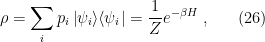
So far everything I’ve reviewed is for zero-temperature field theory; as alluded in the introduction of this post however, finite-temperature is where things get really interesting. Recall from quantum mechanics that a mixed state can be thought of as a statistical ensemble of pure states, so rather than computing expectation values with respect to the vacuum state, we compute them with respect to the mixed state given by the thermal density matrix

where the system, governed by the Hamiltonian , is in any of the states with (classical) probability

Of course, not all mixed states are thermal, but the latter is the correct state to use in the absence of any additional constraints. (One way to think of this is that the mixedness of a quantum state is a measure of our ignorance, which is why pure states are states of minimum entropy). Expectation values of operators with respect to (26) are then ensemble averages at fixed temperature :

Note that we’re in the canonical ensemble (fixed temperature), rather than the microcanonical ensemble (fixed energy), because the energy — that is, the expectation value of the hamiltonian operator 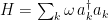— will fluctuate as quanta are created or destroyed. Strictly speaking I should also include the chemical potential, since the number operator also fluctuates, but it doesn’t play any important role in what follows. (The distinction is worth keeping in mind when discussing black hole thermodynamics, where one should use the microcanonical ensemble instead, because the negative specific heat makes the canonical ensemble unstable).

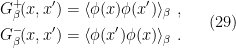
The thermal Green functions (and kernels), which we denote with the subscript , are then obtained by replacing the vacuum expectation value with the expectation value in the thermal state, (28); for example, the Wightman functions become

The aforementioned KMS condition can then be obtained from the Heisenberg equation of motion,

by evolving in Euclidean time by :

where the last step relied on the cyclic property of the trace; similarly for . Thus we arrive at the KMS condition

Note that this is a statement about expectation values of operators in the particular state (26) (indeed, this can easily be formulated for a general observable , we’re just sticking with scalar fields for concreteness; for a slightly more rigorous treatment, with suitable comments about boundedness and whatnot, see for example [2]). More generally however, any state which satisfies (32) is called a KMS state, and describes a system in thermal equilibrium. Similar relations hold for the other Green functions / kernels as well; e.g.,

As an exception to this however, note that since the commutator of free scalar fields is a c-number, in (12) remains unchanged, i.e., .

In arriving at (32), we evolved in imaginary time by an amount given by the (inverse) temperature . This is none other than the usual Wick rotation from Minkowski to Euclidean space, except that the periodicity of the Green functions implies that the Euclidean or thermal time direction is compact, with period . That is, if the original field theory lived on , the finite-temperature field theory lives on , where denotes the (inverse) circumference of the (observe that as , we recover the zero temperature Euclidean theory on ). Thus in general, a Wick rotation in which Euclidean time is periodic makes an intimate connection between QFT and statistical thermodynamics, where the compact direction controls the temperature.

So what does this have to do with black holes, or horizons more generally? As I hope to cover in a future part of this sequence, the spacetime outside a horizon is also described by a thermal state. From the statistical thermodynamics or information theory perspective, one can think of this as due to the fact that we traced over the states on the other side, so the mixed density matrix that now describes the part of the vacuum to which we have access is a reflection of our ignorance. As alluded in the previous paragraph however, the thermodynamic character of the vacuum in the black hole state is already encoded in the periodicity of the Euclidean time direction, and emerges quite neatly in the case of the Schwarzschild black hole,

where is the Schwarzschild radius, and is the metric on the sphere, which we’ll ignore since it just comes along for the ride. Recall from my very first blog post that after Wick rotating to Euclidean time, one can make a coordinate change so that the near-horizon metric becomes

where is the radial direction, and — since these are polar coordinates — takes on the role of the angular coordinate, which must be periodic to avoid a conical singularity; that is, for any integer ,

and thus we identify the period .

As a closing comment, the density matrix for KMS states has deeper relations to the idea of time translation symmetry via Tomita-Takesaki theory, through the modular hamiltonian that generates this 1-parameter family of automorphisms of the algebra of operators in the corresponding region. See for example [3]; this strikes me as a surprisingly under-researched direction, and I hope to revisit it in glorious detail soon.

References

- N. D. Birrell and P. C. W. Davies, Quantum Fields in Curved Space. Cambridge Monographs on Mathematical Physics. Cambridge Univ. Press, Cambridge, UK, 1984. http://www.cambridge.org/mw/academic/subjects/physics/theoretical-physics-and-mathematical-physics/quantum-fields-curved-space?format=PB.
- S. Fulling and S. Ruijsenaars, “Temperature, periodicity and horizons,” Physics Reports 152 no. 3, (1987) 135 – 176.
- A. Connes and C. Rovelli, “Von neumann algebra automorphisms and time-thermodynamics relation in generally covariant quantum theories,” Classical and Quantum Gravity 11 no. 12, (Dec, 1994) 2899–2917, https://arxiv.org/abs/gr-qc/9406019
I really appreciate your notes on this topic. I am a Ph.D student and also major in this field about holography, AdS/CFT, tensor network, black hole information problem and neural networks. I really learned a lot from your notes. Thank you very much.
LikeLike
Thank you very much for your kind and uplifting comment. It’s encouraging to know you got something out of it, especially in this time of academic isolation. Never stop learning!