In the previous post, we introduced mean field theory (MFT) as a means of approximating the partition function for interacting systems. In particular, we used this to determine the critical point at which the system undergoes a phase transition, and discussed the characteristic divergence of the correlation function. In this post, I’d like to understand how recent work in machine learning has leveraged these ideas from statistical field theory to yield impressive training advantages in deep neural networks. As mentioned in part 1, the key feature is the divergence of the correlation length at criticality, which controls the depth of information propagation in such networks.

I’ll primarily follow a pair of very interesting papers [1,2] on random neural nets, where the input (i.e., pre-activation) of neuron in layer is given by

where is some non-linear activation function of the neurons in the previous layer, and is an matrix of weights. The qualifier “random” refers to the fact that the weights and biases are i.i.d. according to the normal distributions

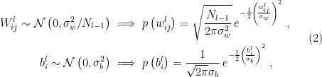
where the factor of has been introduced to ensure that the contribution from the previous layer remains regardless of layer width.

Given this, what is the probability distribution for the inputs ? Treating as fixed, this is a linear combination of independent, normally-distributed variables, so we expect it to be Gaussian as well. Indeed, we can derive this rather easily by considering the characteristic function, which is a somewhat more fundamental way of characterizing probability distributions than the moment and cumulant generating functions we’ve discussed before. For a random variable , the characteristic function is defined as

where in the second equality we assume the probability density (i.e., distribution) function exists. Hence for a Gaussian random variable , we have

A pertinent feature is that the characteristic function of a linear combination of independent random variables can be expressed as a product of the characteristic functions thereof:

where are independent random variables and are some constants. In the present case, we may view each as a constant modifying the random variable , so that

Comparison with (4) then implies that indeed follow a Gaussian,

This is the probability distribution that describes the pre-activations of the neurons in layer . Note that since the neurons are indistinguishable (i.e., all identical), in the large- limit becomes the variance of the distribution of inputs across the entire layer. The MFT approximation is then to simply replace the actual neurons with values drawn from this distribution, which becomes exact in the large- limit (EDIT: there’s a subtlety here, see “MFT vs. CLT” after the references below). For consistency with [1] (and because tracking the -dependence by writing is cumbersome), we’ll introduce the notation  to denote the variance of the pre-activations in layer .

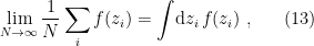
Now, observe that in the large- limit, the average over the activations of the previous layer becomes an integral:

where we’ve used to denote the standard normal Gaussian measure, and we’ve defined so that . That is, we can’t just write

because this makes an assumption on the measure, . Specifically, it assumes that we’re integrating over the real line, whereas we know that in fact lie along a Gaussian. Thus we need a Lebesgue integral (rather than the more familiar Riemann integral) with an appropriate measure—in this case, . (We could alternatively have written , but it’s cleaner to simply rescale things). Substituting this back into (7), we thus obtain a recursion relation for the variance:

which is eqn. (3) of [1]. Very loosely speaking, this describes the spread of information at a single neuron, with smaller values implying a more tightly peaked distribution. We’ll return to the importance of this expression momentarily.

As you might have guessed from all the song-and-dance about correlation functions in part 1 and above, a better probe of information propagation in the network is the correlator of two inputs (in this case, the correlation between different inputs in two identically prepared copies of the network). Let us thus add an additional Latin index to track particular inputs through the network, so that is the value of the neuron in layer in response to the data , is its value in response to data , etc., where the data is fed into the network by setting (here boldface letters denote the entire layer, treated as a vector in ). We then consider the two-point correlator between these inputs at a single neuron:

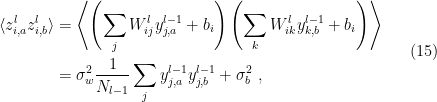
where we have used the fact that 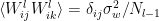, and that the weights and biases are independent with . Note that since , this also happens to be the covariance , which we shall denote in accordance with the notation from [1] introduced above.

As in the single-input case above, we again take the continuum (i.e., large-) limit, whereupon the sum becomes

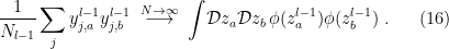
Unlike the previous case however, we can’t just use independent standard Gaussian measures for and , since that would preclude any correlation in the original inputs . Rather, any non-zero correlation in the data will propagate through the network, so the appropriate measure is the bivariate normal distribution,

where the (Pearson) correlation coefficient is defined as

and we have denoted the squared variance in layer corresponding to the input by . If the inputs are uncorrelated (i.e., ), then , and the measure reduces to a product of independent Gaussian variables, as expected. (I say “as expected” because the individual inputs are drawn from a Gaussian. In general however, uncorrelatedness does not necessarily imply independence! The basic reason is that the correlation coefficient is only sensitive to linear relationships between random variables and ; if these are related non-linearly, then it’s possible for them to be dependent () despite being uncorrelated (). See Wikipedia for a simple example of such a case.)

Following [1], the clever trick is then to define new integration variables such that

(Do not confuse the standard normal integration variables with the inputs ; the former are distinguished by the lack of any layer label ). With this substitution, the integral (16) becomes

and thus we obtain the recursion relation for the covariance, cf. eqn. (5) of [1]:

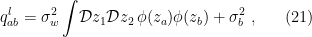
with given by (19). Note that since are Gaussian, their independence (i.e., the fact that ) follows from their uncorrelatedness, ; the latter is easily shown by direct computation, and recalling that .

Now, the interesting thing about the recursion relations (14) and (21) is that they exhibit fixed points for particular values of , , which one can determine graphically (i.e., numerically) for a given choice of non-linear activation . For example, the case is plotted in fig. 1 of [1] (shown below), demonstrating that the fixed point condition

is satisfied for a range of . Therefore, when the parameters of the network (i.e., the distributions (2)) are tuned appropriately, the variance remains constant as signals propagate through the layers. This is useful, because it means that non-zero biases at each layer prevent signals from decaying to zero. Furthermore, provided the non-linearity is concave, the convergence to the fixed point occurs relatively rapidly as a function of depth (i.e., layer ). One can verify this numerically for the case considered above: since , the dynamics ensures convergence to for all initial values. To visualize this, consider the following figure, which I took from [1] ( is their notation for the recursion relation (14)). In the left plot, I’ve added the red arrows illustrating the convergence to the fixed point for . For the particular starting point I chose, it takes about 3 iterations to converge, which is consistent with the plot on the right.

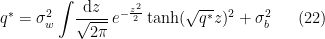
Similarly, the swift convergence to for the variance of individual neurons implies a fixed point for (21). Observe that when , . Hence by dividing (21) by , we have

This equation always has a fixed point at :

where , and we have identified the single-neuron variance , cf. (14), which is .

Let us now ask about the stability of this fixed point. As observed in [1], this is probed by the first derivative evaluated at :

where (the second equality is not obvious; see the derivation at the end of this post if you’re curious). The reason is that for monotonic functions , implies that the curve (23) must approach the unity line from above (i.e., it’s concave, or has a constant slope with a vertical offset at set by the biases), and hence in this case is driven towards the fixed point . Conversely, if , the curve must be approaching this point from below (i.e., it’s convex), and hence in this case is driven away from unity. Depending on the strengths of the biases relative to the weights, the system will then converge to some new fixed point that approaches zero as . (It may help to sketch a few examples, like I superimposed on the left figure above, to convince yourself that this slope/convergence argument works).

The above implies the existence of an order-to-chaos phase transition in the plane: corresponds to the chaotic phase, in which the large random weights cause any correlation between inputs to shrink, while corresponds to the ordered phase, in which the inputs become perfectly aligned and hence . At exactly , the system lies at a critical point, and should therefore be characterized some divergence(s) (recall that, in the limit , a phase transition is defined by the discontinuous change of some quantity; one often hears of an “ order phase transition” if the discontinuity lies in the derivative of the free energy).

We saw in part 1 that at a critical point, the correlation length that governs the fall-off of the two-point correlator diverges. This is the key physics underlying the further development of this mean field framework in [2], who used it to show that random networks are trainable only in the vicinity of this phase transition. Roughly speaking, the intuition is that for such a network to be trainable, information must be able to propagate all the way through the network to establish a relationship between the input (data) and the output (i.e., the evaluation of the cost function) (actually, it needs to go both ways, so that one can backpropagate the gradients through as well). In general, correlations in the input data will exhibit some fall-off behaviour as a function of depth, which limits how far information can propagate through these networks. However, borrowing our physics terminology, we may say that a network at criticality exhibits fluctuations on all scales, so there’s no fall-off behaviour limiting the propagation of information with depth.

So, what is the correlation length in the present problem? In the previous post on mean field theory, we determined this by examining the fall-off of the connected 2-point correlator (i.e., the Green function), which in this case is just . To determine the fall-off behaviour, we expand near the critical point, and examine the difference as (where recall . The limit simply ensures that exist; as shown above, we don’t have to wait that long in practice). This is done explicitly in [2], so I won’t work through all the details here; the result is that upon expanding , one finds the recurrence relation

up to terms of order . This implies that, at least asymptotically, , which one can verify by substituting this into (26) and identifying

Thus is the correlation length that governs the propagation of information — i.e., the decay of the two-point correlator — through the network. And again, we know from our discussion in part 1 that the correlation length diverges at the critical point, which is indeed what happens here: denoting the value of the correlation length at the critical point by , observe that the argument of (27) reduces to (25), i.e.,

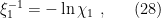
which goes to infinity precisely at the order-to-chaos phase transition, since the latter occurs at exactly .

In practice of course, both and the number of neurons are finite, which precludes a genuine discontinuity at the phase transition (since the partition function is then a finite sum of analytic functions). Nonetheless, provided , we expect that the basic conclusion about trainability above still holds even if the correlation length remains finite. And indeed, the main result of [2] is that at the critical point, not only can information about the inputs propagate all the way through the network, but information about the gradients can also propagate backwards (that is, exploding/vanishing gradients happen only in the ordered/chaotic phases, respectively, but are stable at the phase transition), and consequently these random networks are trainable provided .

Incidentally, you might worry about the validity of these MFT results, given that — as stressed in part 1 — it’s precisely at a critical point that MFT may break down, due to the relevance of higher-order terms that the approximation ignores. But in this case, we didn’t neglect anything: we saw in (7) that the distribution of inputs already follows a Gaussian, so the only “approximation” lies in ignoring any finite-size effects associated with backing away from the limit (EDIT: actually, this isn’t true! See “MFT vs. CLT” below).

The application of MFT to neural networks is actually a rather old idea, with the presence of an order-to-chaos transition known in some cases since at least the 1980’s [3]. More generally, the idea that the critical point may offer unique benefits to computation has a long and eclectic history, dating back to an interesting 1990 paper [4] on cellular automata that coined the phrase “computation at the edge of chaos”. However, only in the past few years has this particular interdisciplinary ship really taken off, with a number of interesting papers demonstrating the power of applying physics to deep learning. The framework developed in [1,2] that I’ve discussed here has already been generalized to convolutional [5] and recurrent [6,7] neural networks, where one again finds that initializing the network near the phase transition results in significant improvements in training performance. It will be exciting to see what additional insights we can discover in the next few years.

---

The second equality in (25), namely

is not obvious, but requires an exercise in basic calculus. Since all the functional dependence on — denoted simply here for brevity — is contained in (cf.(19)), we have from (23)

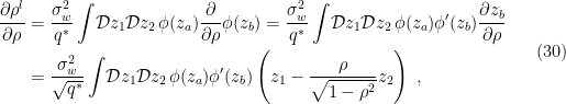
where the prime denotes the derivative of with respect to its argument. We now use the hint given in the appendix of [1], namely that for the standard Gaussian measure, integration by parts allows us to write . We therefore have the identities

and

where in the last step we have again applied integration by parts over the Gaussian measure. Substituting these results into (30), we find

If we evaluate this at , we can integrate freely over , whereupon the second term vanishes,

and the first returns the claimed result:

---

MFT vs. CLT (edit 2021-12-09)

Throughout this post, I referred to the approximation employed in [1,2] as MFT, since they and related works in the machine learning literature advertise it under this name. It turns out however that this isn’t quite right: the results above actually follow directly from the central limit theorem (CLT), which — perhaps surprisingly — is not necessarily the same as MFT. I discovered this together with my excellent collaborator Kevin Grosvenor while working on the nascent NN-QFT correspondence. I might write a dedicated blog article about this at some point, but the basic idea is to develop the connections between physics and machine learning that I’ve alluded to in various places here in more detail, and use techniques from QFT in particular to understand deep neural networks.

In our latest paper, we made this correspondence concrete by explicitly constructing the QFT corresponding to a general class of networks including both recurrent and feedforward architectures. The MFT approximation corresponds to the leading saddle point of the theory, as I’ve explained before. But we can also compute perturbative corrections in , the ratio of depth to width (this works for most deep networks of practical interest, which typically have ). Finite-width corrections appear at , which physically correspond to effective interactions that arise upon marginalizing over hidden degrees of freedom; see my post on deep learning and the renormalization group for details.

However, we also discovered an correction to the MFT (i.e., tree level) result, which is independent of network size, and therefore survives in the limit. Physically, this corresponds to fluctuations in the ensemble of random networks under study; some intuition for this is given in section 5 of the aforementioned paper. Since MFT ignores all fluctuations (not just those arising at finite width), it fails to capture this contribution. Results from the CLT might implicitly include this effect, but this has yet to be worked-out in detail.

References

- B. Poole, S. Lahiri, M. Raghu, J. Sohl-Dickstein, and S. Ganguli, “Exponential expressivity in deep neural networks through transient chaos,” arXiv:1606.05340 [stat.ML].
- S. S. Schoenholz, J. Gilmer, S. Ganguli, and J. Sohl-Dickstein, “Deep Information Propagation,” arXiv:1611.01232 [stat.ML].
- H. Sompolinsky, A. Crisanti, and H. J. Sommers, “Chaos in random neural networks,” Phys. Rev. Lett. 61 (Jul, 1988) 259–262.
- C. G. Langton, “Computation at the edge of chaos: Phase transitions and emergent computation,” Physica D: Nonlinear Phenomena 42 no. 1, (1990) 12 – 37.
- L. Xiao, Y. Bahri, J. Sohl-Dickstein, S. S. Schoenholz, and J. Pennington, “Dynamical Isometry and a Mean Field Theory of CNNs: How to Train 10,000-Layer Vanilla Convolutional Neural Networks,” arXiv:1806.05393 [stat.ML].
- M. Chen, J. Pennington, and S. S. Schoenholz, “Dynamical Isometry and a Mean Field Theory of RNNs: Gating Enables Signal Propagation in Recurrent Neural Networks,” arXiv:1806.05394 [stat.ML].
- D. Gilboa, B. Chang, M. Chen, G. Yang, S. S. Schoenholz, E. H. Chi, and J. Pennington, “Dynamical Isometry and a Mean Field Theory of LSTMs and GRUs,” arXiv:1901.08987 [cs.LG].