
In recent years, a number of works have pointed to similarities between deep learning (DL) and the renormalization group (RG) [1-7]. This connection was originally made in the context of certain lattice models, where decimation RG bears a superficial resemblance to the structure of deep networks in which one marginalizes over hidden degrees of freedom. However, the relation between DL and RG is more subtle than has been previously presented. The “exact mapping” put forth by [2], for example, is really just a formal analogy that holds for essentially any hierarchical model! That’s not to say there aren’t deeper connections between the two: in my earlier post on RBMs for example, I touched on how the cumulants encoding UV interactions appear in the renormalized couplings after marginalizing out hidden degrees of freedom, and we’ll go into this in much more detail below. But it’s obvious that DL and RG are functionally distinct: in the latter, the couplings (i.e., the connection or weight matrix) are fixed by the relationship between the hamiltonian at different scales, while in the former, these connections are dynamically altered in the training process. There is, in other words, an important distinction between structure and dynamics which seems to have been overlooked. Understanding both these aspects is required to truly understand why deep learning “works”, but “learning” itself properly refers to the latter.
That said, structure is the first step to dynamics, so I wanted to see how far one could push the analogy. To that end, I started playing with simple Gaussian/Bernoulli RBMs, to see whether understanding the network structure — in particular, the appearance of hidden cumulants, hence the previous post in this two-part sequence — would shed light on, e.g., the hierarchical feature detection observed in certain image recognition tasks, the propagation of structured information more generally, or the relevance of criticality to both deep nets and biological brains. To really make the RG analogy precise, one would ideally like a beta function for the network, which requires a recursion relation for the couplings. So my initial hope was to derive an expression for this in terms of the cumulants of the marginalized neurons, and thereby gain some insight into how correlations behave in these sorts of hierarchical networks.
To start off, I wanted a simple model that would be analytically solvable while making the analogy with decimation RG completely transparent. So I began by considering a deep Boltzmann machine (DBM) with three layers: a visible layer of Bernoulli units 


where on the second line I’ve switched to the more convenient vector notation; the dot product between vectors is implicit, i.e., 


The joint distribution function describing the state of the machine is
![\displaystyle p(x,y,z)=Z^{-1}e^{-\beta H(x,y,z)}~, \quad\quad Z[\beta]=\prod_{i=1}^n\sum_{x_i=\pm1}\int\!\mathrm{d}^my\mathrm{d}^pz\,e^{-\beta H(x,y,z)}~, \ \ \ \ \ (2)](https://s0.wp.com/latex.php?latex=%5Cdisplaystyle+p%28x%2Cy%2Cz%29%3DZ%5E%7B-1%7De%5E%7B-%5Cbeta+H%28x%2Cy%2Cz%29%7D%7E%2C+%5Cquad%5Cquad+Z%5B%5Cbeta%5D%3D%5Cprod_%7Bi%3D1%7D%5En%5Csum_%7Bx_i%3D%5Cpm1%7D%5Cint%5C%21%5Cmathrm%7Bd%7D%5Emy%5Cmathrm%7Bd%7D%5Epz%5C%2Ce%5E%7B-%5Cbeta+H%28x%2Cy%2Cz%29%7D%7E%2C+%5C+%5C+%5C+%5C+%5C+%282%29&bg=ffffff&fg=000000&s=0&c=20201002)
where 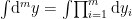


In order to establish a relationship between couplings at each energy scale, we then define the hamiltonian on the remaining, lower-energy degrees of freedom 


This is a simple multidimensional Gaussian integral:

where in the present case 


The key point to note is that the interactions between the intermediate degrees of freedom

The cumulant generating function for 

cf. eqn. (4) in the previous post. So by choosing 

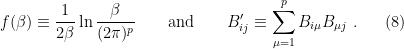
and may therefore express (7) as

From the cumulant expansion in the aforementioned eqn. (4), in which the 

For the Gaussian prior (9), one immediately sees from (10) that all cumulants except for 
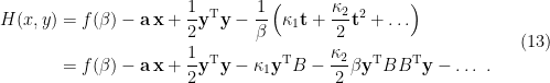
Now, let’s repeat this process to obtain the marginalized distribution of purely visible units

Of course, this is just another edition of (6), but now with 

![\displaystyle \begin{aligned} p(x)&=Z^{-1}\sqrt{\frac{(2\pi)^m}{\beta\left(1-|B'|\right)}}\mathrm{exp}\left[-\beta\left( f(\beta)-\mathbf{a}\mathbf{x}+\frac{1}{2}\mathbf{x}^\mathrm{T} A\left(\mathbf{1}-B'\right)^{-1}A^\mathrm{T}\mathbf{x}\right)\right]\\ &=Z^{-1}\sqrt{\frac{(2\pi)^m}{\beta\left(1-|B'|\right)}}\mathrm{exp}\left[-\beta\left( f(\beta)-\mathbf{a}\mathbf{x}+\frac{1}{2}\mathbf{x}^\mathrm{T} A'\mathbf{x}\right)\right] \end{aligned} \ \ \ \ \ (15)](https://s0.wp.com/latex.php?latex=%5Cdisplaystyle+%5Cbegin%7Baligned%7D+p%28x%29%26%3DZ%5E%7B-1%7D%5Csqrt%7B%5Cfrac%7B%282%5Cpi%29%5Em%7D%7B%5Cbeta%5Cleft%281-%7CB%27%7C%5Cright%29%7D%7D%5Cmathrm%7Bexp%7D%5Cleft%5B-%5Cbeta%5Cleft%28+f%28%5Cbeta%29-%5Cmathbf%7Ba%7D%5Cmathbf%7Bx%7D%2B%5Cfrac%7B1%7D%7B2%7D%5Cmathbf%7Bx%7D%5E%5Cmathrm%7BT%7D+A%5Cleft%28%5Cmathbf%7B1%7D-B%27%5Cright%29%5E%7B-1%7DA%5E%5Cmathrm%7BT%7D%5Cmathbf%7Bx%7D%5Cright%29%5Cright%5D%5C%5C+%26%3DZ%5E%7B-1%7D%5Csqrt%7B%5Cfrac%7B%282%5Cpi%29%5Em%7D%7B%5Cbeta%5Cleft%281-%7CB%27%7C%5Cright%29%7D%7D%5Cmathrm%7Bexp%7D%5Cleft%5B-%5Cbeta%5Cleft%28+f%28%5Cbeta%29-%5Cmathbf%7Ba%7D%5Cmathbf%7Bx%7D%2B%5Cfrac%7B1%7D%7B2%7D%5Cmathbf%7Bx%7D%5E%5Cmathrm%7BT%7D+A%27%5Cmathbf%7Bx%7D%5Cright%29%5Cright%5D+%5Cend%7Baligned%7D+%5C+%5C+%5C+%5C+%5C+%2815%29&bg=ffffff&fg=000000&s=0&c=20201002)
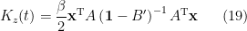
where we have defined 


 are given in (8).
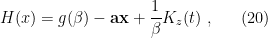
Again we see that marginalizing out UV information induces new couplings between IR degrees of freedom; in particular, the hamiltonian 


(where, since 

with 

To summarize, the sequential flow from UV (hidden) to IR (visible) distributions is, from top to bottom,
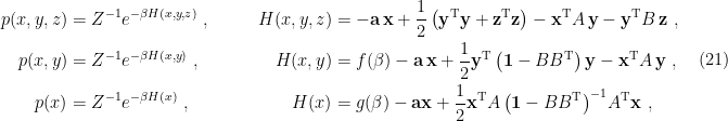
where upon each marginalization, the new hamiltonian gains additional interaction terms/couplings governed by the cumulants of the UV prior (where “UV” is defined relative to the current cutoff scale, i.e., 


As an aside, note that at each level, fixing the form (4), (16) is equivalent to imposing that the partition function remain unchanged. Ultimately, this is required in order to preserve low-energy correlation functions. The two-point correlator 


Failure to satisfy this requirement amounts to altering the theory at each energy scale, in which case there would be no consistent renormalization group relating them. In information-theoretic terms, this would represent an incorrect Bayesian inference procedure.
Despite (or perhaps, because of) its simplicity, this toy model makes manifest the fact that the RG prescription is reflected in the structure of the network, not the dynamics of learning per se. Indeed, Gaussian units aside, the above is essentially nothing more than real-space decimation RG on a 1d lattice, with a particular choice of couplings between “spins” 

Nonetheless, there’s clearly an intimate parallel between RG and hierarchical Bayesian modeling at play here. As mentioned above, I’d originally hoped to derive something like a beta function for the cumulants, to see what insights theoretical physics and machine learning might yield to one another at this information-theoretic interface. Unfortunately, while one can see how the higher UV cumulants from
Fortunately, after banging my head against this for a month, I learned of a recent paper [8] that derives exactly the sort of cumulant relation I was aiming for, at least in the case of generic lattice models. The key is to not assume a priori which degrees of freedom will be considered UV/hidden vs. IR/visible. That is, when I wrote down the joint distribution (2), I’d already distinguished which units would survive each marginalization. While this made the parallel with the familiar decimation RG immediate — and the form of (1) made the calculations simple to perform analytically — it’s actually a bit unnatural from both a field-theoretic and a Bayesian perspective: the degrees of freedom that characterize the theory in the UV may be very different from those that we observe in the IR (e.g., strings vs. quarks vs. hadrons), so we shouldn’t make the distinction 

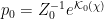
where 


Two words of notational warning ere we proceed: first, there is a sign error in eqn. (1) of [8] (in version 1; the negative in the exponent has been absorbed into 
Let us now repeat the above analysis in this more general framework. The real-space RG prescription consists of coarse-graining 


where 


So far, so familiar, but now comes the trick: [8] split the hamiltonian 


Let us denote a block of hidden units by 


where 

Now, getting from this to the first line of eqn. (13) in [8] is a bit of a notational hazard. We must suppose that for each block 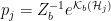


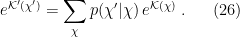
Thus we see that we can insert a factor of 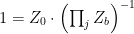

and 

where the expectation value is defined with respect to the conditional distribution 

which one clearly recognizes as a generalization of (12): 


Within expectation values, 


where 
This is great, but we’re not quite finished, since we’d still like to determine the renormalized couplings in terms of the cumulants, as I did in the simple Gaussian DBM above. This requires expressing the new hamiltonian in the same form as the old, which allows one to identify exactly which contributions from the UV degrees of freedom go where. (See for example chapter 13 of [9] for a pedagogical exposition of this decimation RG procedure for the 1d Ising model). For the class of lattice models considered in [8] — by which I mean, real-space decimation with the imposition of a buffer zone — one can write down a formal expression for the canonical form of the hamiltonian, but expressions for the renormalized couplings themselves remain model-specific.
There’s more cool stuff in the paper [8] that I won’t go into here, concerning the question of “optimality” and the behaviour of mutual information in these sorts of networks. Suffice to say that, as alluded in the previous post, the intersection of physics, information theory, and machine learning is potentially rich yet relatively unexplored territory. While the act of learning itself is not an RG in a literal sense, the two share a hierarchical Bayesian language that may yield insights in both directions, and I hope to investigate this more deeply (pun intended) soon.
References
[1] C. Beny, “Deep learning and the renormalization group,” arXiv:1301.3124.
[2] P. Mehta and D. J. Schwab, “An exact mapping between the Variational Renormalization Group and Deep Learning,” arXiv:1410.3831.
[3] H. W. Lin, M. Tegmark, and D. Rolnick, “Why Does Deep and Cheap Learning Work So Well?,” arXiv:1608.08225.
[4] S. Iso, S. Shiba, and S. Yokoo, “Scale-invariant Feature Extraction of Neural Network and Renormalization Group Flow,” arXiv:1801.07172.
[5] M. Koch-Janusz and Z. Ringel, “Mutual information, neural networks and the renormalization group,” arXiv:1704.06279.
[6] S. S. Funai and D. Giataganas, “Thermodynamics and Feature Extraction by Machine Learning,” arXiv:1810.08179.
[7] E. Mello de Koch, R. Mello de Koch, and L. Cheng, “Is Deep Learning an RG Flow?,” arXiv:1906.05212.
[8] P. M. Lenggenhager, Z. Ringel, S. D. Huber, and M. Koch-Janusz, “Optimal Renormalization Group Transformation from Information Theory,” arXiv:1809.09632.
[9] R. K. Pathria, Statistical Mechanics. 1996. Butterworth-Heinemann, Second edition.

I was just curious to know what happens if we use convolutional neural networks to process the data. Will it make a considerable difference? For example in [2], wouldn’t it have been better to use convoluted RBMs (assuming such a thing exists)?
LikeLike
Pingback: Big AGI Breakthrough: Leveling the Playing Field - Themesis, Inc.