In several recent posts, I explored various ideas that lie at the interface of physics, information theory, and machine learning:

• We’ve seen, à la Jaynes, how the concepts of entropy in statistical thermodynamics and information theory are unified, perhaps the quintessential manifestation of the intimate relationship between the two.
• We applied information geometry to Boltzmann machines, which led us to the formalization of “learning” as a geodesic in the abstract space of machines.
• In the course of introducing VAEs, we saw that the Bayesian inference procedure can be understood as a process which seeks to minimizes the variational free energy, which encodes the divergence between the approximate and true probability distributions.
• We examined how the (dimensionless) free energy serves as a generating function for the cumulants from probability theory, which manifest as the connected Green functions from quantum field theory.
• We also showed how the cumulants from hidden priors control the higher-order interactions between visible units in an RBM, which underlies their representational power.
• Lastly, we turned a critical eye towards the analogy between deep learning and the renormalization group, through a unifying Bayesian language in which UV degrees of freedom correspond to hidden variables over which a low-energy observer must marginalize.

Collectively, this led me to suspect that ideas along these lines — in particular, the link between variational Bayesian inference and free energy minimization in hierarchical models — might provide useful mathematical headway in our attempts to understand learning and intelligence in both minds and machines. It turns out this has been explored before by many scientists; at least in the context of biological brains, the most well-known is probably the approach by the neuroscientist Karl Friston, which provides a convenient starting point for exploring these ideas.

The aptly-named free energy principle (for the brain) is elaborated upon in a series of about ten papers spanning as many years. I found [1-5] most helpful, but insofar as a great deal of text is copied verbatim (yes, really; never trust the h-index) it doesn’t really matter which one you read. I’m going to mostly draw from [3], because it seems the earliest in which the basic idea is fleshed-out completely. Be warned however that the notation varies slightly from paper to paper, and I find his distinction between states and parameters rather confusingly fuzzy; but we’ll make this precise below.

The basic idea is actually quite simple, and proceeds from the view of the brain as a Bayesian inference machine. In a nutshell, the job of the brain is to infer, as accurately as possible, the probability distribution representing the world (i.e., to build a model that best accords with sensory inputs). In a sense, the brain itself is a probabilistic model in this framework, so the goal is to bring this internal model of the world in line with the true, external one. But this is exactly the same inference procedure we’ve seen before in the context of VAEs! Thus the free energy principle is just the statement that the brain minimizes the variational free energy between itself (that is, its internal, approximate model) and its sensory inputs—or rather, the true distribution that generates them.

To elucidate the notation involved in formulating the principle, we can make an analogy with VAEs. In this sense, the goal of the brain is to construct a map between our observations (i.e., sensory inputs ) and the underlying causes (i.e., the environment state ). By Bayes’ theorem, the joint distribution describing the model can be decomposed as

The first factor on the right-hand side is the likelihood of a particular sensory input given the current state of the environment , and plays the role of the decoder in this analogy, while the second factor is the prior distribution representing whatever foreknowledge the system has about the environment. The subscript denotes the variational or “action parameters” of the model, so named because they parametrize the action of the brain on its substrate and surroundings. That is, the only way in which the system can change the distribution is by acting to change its sensory inputs. Friston denotes this dependency by (with different variables), but as alluded above, I will keep to the present notation to avoid conflating state/parameter spaces.

Continuing this analogy, the encoder is then a map from the space of sensory inputs to the space of environment states (as modelled by the brain). As in the case of VAEs however, this is incomputable in practice, since we (i.e., the brain) can’t evaluate the partition function . Instead, we construct a new distribution for the conditional probability of environment states given a particular set of sensory inputs . The variational parameters for this ensemble control the precise hamiltonian that defines the distribution, i.e., the physical parameters of the brain itself. Depending on the level of resolution, these could represent, e.g., the firing status of all neurons, or the concentrations of neurotransmitters (or the set of all weights and biases in the case of artificial neural nets).

Obviously, the more closely approximates , the better our representation — and hence, the brain’s predictions — will be. As we saw before, we quantify this discrepancy by the Kullback-Leibler divergence

which we can re-express in terms of the variational free energy

where the subscripts denote the conditional distributions , . On the far right-hand side, is the energy or hamiltonian for the ensemble (with partition function ), and is the entropy of (see the aforementioned post for details).

However, at this point we must diverge from our analogy with VAEs, since what we’re truly after is a model of the state of the world which is independent of our current sensory inputs. Consider that from a selectionist standpoint, a brain that changes its environmental model when a predator temporarily moves out of sight is less likely to pass on the genes for its construction! Said differently, a predictive model of reality will be more successful when it continues to include the moon, even when nobody looks at it. Thus instead of , we will compare with the ensemble density , where — unlike in the case of or — we have denoted the variational parameters explicitly, since they will feature crucially below. Note that is not the same as (and similarly, whatever parameters characterize the marginals , cannot be identified with ). One way to see this is by comparison with our example of renormalization in deep networks, where the couplings in the joint distribution (here, in ) get renormalized after marginalizing over some degrees of freedom (here, in , after marginalizing over all possible sensory inputs ). Friston therefore defines the variational free energy as

where we have used a curly to distinguish this from above, and note that the subscript (no vertical bar) denotes that expectation values are computed with respect to the distribution . The first equality expresses as the log-likelihood of sensory inputs given the state of the environment, minus an error term that quantifies how far the brain’s internal model of the world is from the model consistent with our observations, , cf. (1). Equivalent, comparing with (2) (with in place of ), we’re interested in the Kullback-Leibler divergence between the brain’s model of the external world, , and the conditional likelihood of a state therein given our sensory inputs, . Thus we arrive at the nutshell description we gave above, namely that the principle is to minimize the difference between what is and what we think there is. As alluded above, there is a selectionist argument for this principle, namely that organisms whose beliefs accord poorly with reality tend not to pass on their genes.

As an aside, it is perhaps worth emphasizing that both of these variational free energies are perfectly valid: unlike the Helmholtz free energy, which is uniquely defined, one can define different variational free energies depending on which ensembles one wishes to compare, provided it admits an expression of the form for some energy and entropy (in case it wasn’t clear by now, we’re working with the dimensionless or reduced free energy, equivalent to setting ; the reason for this general form involves a digression on Legendre transforms). Comparing (4) and (3), one sees that the difference in this case is simply a difference in entropies and expectation values with respect to prior vs. conditional distributions (which makes sense, since all we did was replace the latter by the former in our first definition).

Now, viewing the brain as an inference machine means that it seeks to optimize its predictions about the world, which in this context, amounts to minimizing the free energy by varying the parameters . As explained above, corresponds to the actions the system can take to alter its sensory inputs. From the first equality in (4), we see that the dependence on the action parameters is entirely contained in the log-likelihood of sensory inputs: the second, Kullback-Leibler term contains only priors (cf. our discussion of gradient descent in VAEs). This, optimizing the free energy with respect to means that the system will act in such a way as to fulfill its expectations with regards to sensory inputs. Friston neatly summarizes this philosophy as the view that “we may not interact with the world to maximize our reward but simply to ensure it behaves as we think it should” [3]. While this might sound bizarre at first glance, the key fact to bear in mind is that the system is limited in the actions it can perform, i.e., in its ability to adapt. In other words, a system with low free energy is per definition adapting well to changes in its environment or its own internal needs, and therefore is positively selected for relative to systems whose ability to model and adapt to their environment is worse (higher free energy).

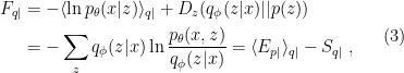
What about optimization with respect to the other set of variational parameters, ? As mentioned above, these correspond to the physical parameters of the system itself, so this corresponds to adjusting the brain’s internal parameters — connection strengths, neurotransmitter levels, etc. — to ensure that our perceptions are as accurate as possible. By applying Bayes rule to the joint distribution , we can re-arrange the expression for the free energy to isolate this dependence in a single Kullback-Leibler term:

where we have used the fact that . This form of the expression shows clearly that minimization with respect to directly corresponds to minimizing the Kullback-Leibler divergence between the brain’s internal model of the world, , and the posterior probability of the state giving rise to its sensory inputs, . That is, in the limit where the second, Kullback-Leibler term vanishes, we are correctly modelling the causes of our sensory inputs. The selectionist interpretation is that systems which are less capable of accurately modelling their environment by correctly adjusting internal, “perception parameters” will have higher free energy, and hence will be less adept in bringing their perceptions in line with reality.

Thus far everything is quite abstract and rather general. But things become really interesting when we apply this basic framework to hierarchical models with both forward and backwards connections — such as the cerebral cortex — which leads to “recurrent dynamics that self-organize to suppress free energy or prediction error, i.e., recognition dynamics” [3]. In fact, Friston makes the even stronger argument that it is precisely the inability to invert the recognition problem that necessitates backwards (as opposed to purely feed-forwards) connections. In other words, the selectionist pressure to accurately model the (highly non-linear) world requires that brains evolve top-down connections from higher to lower cortical layers. Let’s flesh this out in a bit more detail.

Recall that is the space of environmental states as modelled by the brain. Thus we can formally associate the encoder, , with forwards connections, which propagate sensory data up the cortical hierarchy; Friston refers to this portion as the recognition model. That is, the recognition model should take a given data point , and return the likelihood of a particular cause (i.e., world-state) . In general however, the map from causes to sensory inputs — captured by the so-called generative model — is highly non-linear, and the brain must essentially invert this map to find contextually invariant causes (e.g., the continued threat of a predator even when it’s no longer part of our immediate sensory input). This is the intractable problem of computing the partition function above, the workaround for which is to instead postulate an approximate recognition model , whose parameters are encoded in the forwards connections. The role of the generative model is then to modulate sensory inputs (or their propagation and processing) based on the prevailing belief about the environment’s state, the idea being that these effects are represented in backwards (and lateral) connections. Therefore, the role of these backwards or top-down connections is to modulate forwards or bottom-up connections, thereby suppressing prediction error, which is how the brain operationally minimizes its free energy.

The punchline is that backwards connections are necessary for general perception and recognition in hierarchical models. As mentioned above, this is quite interesting insofar as it offers, on the one hand, a mathematical explanation for the cortical structure found in biological brains, and on the other, a potential guide to more powerful, neuroscience-inspired artificial intelligence.

There are however a couple technical exceptions to this claim of necessity worth mentioning, which is why I snuck in the qualifier “general” in the punchline above. If the abstract generative model can be inverted exactly, then there’s no need for (expensive and time-consuming) backwards connections, because one can obtain a perfectly suitable recognition model that reliably predicts the state of the world given sensory inputs, using a purely feed-forward network. Mathematically, this corresponds to simply taking in (4) (i.e., zero Kullback-Leibler divergence (2)), whereupon the free energy reduces to the negative log-likelihood of sensory inputs,

where we have used the fact that . Since real-world models are generally non-linear in their inputs however, invertibility is not something one expects to encounter in realistic inference machines (i.e., brains). Indeed, our brains evolved under strict energetic and space constraints; there simply isn’t enough processing power to brute-force the problem by using dedicated feed-forward networks for all our recognition needs. The other important exception is when the recognition process is purely deterministic. In this case one replaces by a Kronecker delta function , so that upon performing the summation, the inferred state becomes a deterministic function of the inputs . Then the second expression for in (4) becomes the negative log-likelihood of the joint distribution

where we have used the fact that . Note that the invertible case, (6), corresponds to maximum likelihood estimation (MLE), while the deterministic case (7) corresponds to so-called maximum a posteriori estimation (MAP), the only difference being that the latter includes a weighting based on the prior distribution . Neither requires the conditional distribution , and so skirts the incomputability issue with the path integral above. The reduction to these familiar machine learning metrics for such simple models is reasonable, since only in relatively contrived settings does one ever expect deterministic/invertible recognition.

In addition to motivating backwards connections, the hierarchical aspect is important because it allows the brain to learn its own priors through a form of empirical Bayes. In this sense, the free energy principle is essentially an elegant (re)formulation of predictive coding. Recall that when we introduced the generative model in the form of the decoder in (1), we also necessarily introduced the prior distribution : the liklihood of a particular sensory input given (our internal model of) the state of the environment (i.e., the cause) only makes sense in the context of the prior distribution of causes. Where does this prior distribution come from? In artificial models, we can simply postulate some (e.g., Gaussian or informative) prior distribution and proceed to train the model from there. But a hierarchical model like the brain enables a more natural option. To illustrate the basic idea, consider labelling the levels in such a cortical hierarchy by , where 0 is the bottom-most layer and is the top-most layer. Then denotes sensory data at the corresponding layer; i.e., corresponds to raw sensory inputs, while corresponds to the propagated input signals after all previous levels of processing. Similarly, let denote the internal model of the state of the world assembled (or accessible at) the layer. Then

i.e., the prior distribution implicitly depends on the knowledge of the state at all previous levels, analogous to how the IR degrees of freedom implicitly depend on the marginalized UV variables. The above expression can be iterated recursively until we reach . For present purposes, this can be identified with , since at the bottom-most level of the hierarchy, there’s no difference between the raw sensory data and the inferred state of the world (ignoring whatever intralayer processing might take place). In this (empirical Bayesian) way, the brain self-consistently builds up higher priors from states at lower levels.

The various works by Friston and collaborators go into much more detail, of course; I’ve made only the crudest sketch of the basic idea here. In particular, one can make things more concrete by examining the neural dynamics in such models, which some of these works seek to explore via something akin to a mean field theory (MFT) approach. I’d originally hoped to have time to dive into this in detail, but a proper treatment will have to await another post. Suffice to say however that an approach along the lines of the free energy principle may provide an elegant formulation which, as in the other topics mentioned at the beginning of this post, allows us to apply ideas from theoretical physics to understand the structure and dynamics of neural networks, and may even prove a fruitful mathematical framework for both theoretical neuroscience and (neuro-inspired) artificial intelligence.

References:

[1] K. Friston, “Learning and inference in the brain,” Neural Networks (2003) .

[2] K. Frison, “A theory of cortical responses,” Phil. Trans. R. Soc. B (2005) .

[3] K. Friston, J. Kilner, and L. Harrison, “A free energy principle for the brain,” J. Physiology (Paris) (2006) .

[4] K. J. Friston and K. E. Stephan, “Free-energy and the brain,” Synthese (2007) .

[5] K. Friston, “The free-energy principle: a unified brain theory?,” Nature Rev. Neuro. (2010) .