What is entropy?

You should call it entropy, for two reasons. In the first place your uncertainty function has been used in statistical mechanics under that name, so it already has a name. In the second place, and more important, no one really knows what entropy really is, so in a debate you will always have the advantage.

— John von Neumann to Claude Shannon, as to what the latter should call his uncertainty function.

I recently read the classic article [1] by Jaynes, which elucidates the relationship between subjective and objective notions of entropy—that is, between the information-theoretic notion of entropy as a reflection of our ignorance, and the thermodynamic notion of entropy as a measure of the statistical microstates of a system. These two notions are formally identical, and can be written

$\displaystyle S=-\sum_ip_i\ln p_i~, \ \ \ \ \ (1)$

where ${p_i}$ is the probability of the ${i^\mathrm{th}}$ outcome/microstate. However, as Jaynes rightfully stresses, the fact that these concepts share the same mathematical form does not necessarily imply any relation between them. Nonetheless, a physicist cannot resist the intuitive sense that there must be some deeper relationship lurking beneath the surface. And indeed, Jaynes paper [1] makes it beautifully clear that in fact these distinct notions are referencing the same underlying concept—though I may differ from Jaynes in explaining precisely how the subjective/objective divide is crossed.

(As an aside, readers without a theoretical physics background may be confused by the fact that the thermodynamic entropy is typically written with a prefactor ${k_B=1.381\times 10^{-23}J/K}$ , known as Boltzmann’s constant. This is merely a compensatory factor, to account for humans’ rather arbitrary decision to measure temperatures relative to the freezing point of water at atmospheric pressure. Being civilized people, we shall instead work in natural units, in which ${k_B=1}$ .)

As a prelude, let us first explain what entropy has to do with subjective uncertainty. That is, why is (1) a sensible/meaningful/well-defined measure of the information we have available? Enter Claude Shannon, whose landmark paper [2] proved, perhaps surprisingly, that (1) is in fact the unique, unambiguous quantification of the “amount of uncertainty” represented by a discrete probability distribution! Jaynes offers a more intuitive proof in his appendix A [1], which proceeds as follows. Suppose we have a variable ${x}$ , which assumes any of the discrete values ${(x_1,\ldots,x_n)}$ . These could represent, e.g., particular outcomes or measurement values. To each ${x_i}$ , we associated the corresponding probability ${p_i\in(p_1,\ldots,p_n)}$ , with ${\sum\nolimits_ip_i=1}$ . The question is then whether one can find a function ${H(p_1,\ldots,p_n)}$ which uniquely quantifies the amount of uncertainty represented by this probability distribution. Remarkably, Shannon showed [2] that this can indeed be done, provided ${H}$ satisfies the following three properties:

${H}$ is a continuous function of ${p_i}$ .
If all ${p_i}$ are equal, then ${p_i=1/n}$ (since probabilities sum to 1), and ${A(n)\equiv H(1/n,\ldots,1/n)}$ is a monotonically increasing function of ${n}$ .
If we decompose an event into sub-events, then the original value of ${H}$ must be the weighted sum of the individual values of ${H}$ for each composite event.

The first requirement simply ensures that ${H}$ is well-defined. The second encodes the fact that if all events are equally likely, then the uncertainty increases monotonically with the number of events. The third property is referred to as the composition law by Jaynes, and is easily explained with the help of figure 6 in Shannon’s paper [2], which I’ve reproduced here: entropy-12 On the left, we have three probabilities ${p_1\!=\!\tfrac{1}{2}}$ , ${p_2\!=\!\tfrac{1}{3}}$ , and ${p_3\!=\!\tfrac{1}{6}}$ , so the uncertainty for this distribution is given by ${H\!\left(\tfrac{1}{2},\tfrac{1}{3},\tfrac{1}{6}\right)}$ . On the right, we’ve coarse-grained the system such that at the highest level (that is, the left-most branch), we have two equally likely outcomes, and hence uncertainty ${H\!\left(\tfrac{1}{2},\tfrac{1}{2}\right)}$ . However, this represents a different state of knowledge than the original ${H}$ , insofar as it disregards the fine-grained information in the lower branch. Obviously, our uncertainty function should not change simply because we’ve chosen to group certain clusters of events together. Thus in order for ${H}$ to be invariant under this composition, we must have

$\displaystyle H\!\left(\tfrac{1}{2},\tfrac{1}{3},\tfrac{1}{6}\right)=H\!\left(\tfrac{1}{2},\tfrac{1}{2}\right)+\tfrac{1}{2}H\!\left(\tfrac{2}{3},\tfrac{1}{3}\right)~, \ \ \ \ \ (2)$

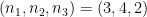
where the ${\tfrac{1}{2}}$ prefactor is the probabilistic weight associated with this composition of events.

To generalize this, it is convenient to represent the probabilities as rational fractions,

$\displaystyle p_i=\frac{n_i}{\sum n_i}~,\quad\quad n_i\in\mathbb{Z}_+~. \ \ \ \ \ (3)$

(The fact that ${H}$ is continuous enables us to make this assumption without loss of generality). This enables us to fix the form of ${H}$ by applying the composition law to the case in which we coarse-grain ${n}$ equally likely alternatives into clusters of size ${n_i}$ , which results in the requirement

$\displaystyle A\left(\sum\nolimits_in_i\right)=H(p_1,\ldots,p_n)+\sum\nolimits_i p_iA(n_i)~. \ \ \ \ \ (4)$

To see this, consider the example given by Jaynes, in which we take ${n=3}$ , and let ${(n_1,n_2,n_3)=(3,4,2)}$ . If all ${\sum_i n_i=9}$ outcomes are equally likely, then the uncertainty, given by the left-hand side of (4), is ${A(9)}$ . As in the previous example, we want this uncertainty to be preserved under coarse-graining, where in this case we group the possible outcomes into ${n=3}$ clusters of size ${n_i}$ , as illustrated in the figure below:

entropy-3

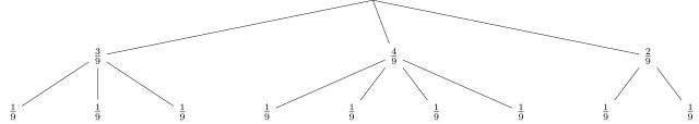
Thus we see that at the highest level, the uncertainty — had we thrown away the fine-grained information in each cluster — is ${H(p_1,p_2,p_3)=H\left(\tfrac{3}{9},\tfrac{4}{9},\tfrac{2}{9}\right)}$ . The second term on the right-hand side of (4) is then the weighted value of ${H}$ for each cluster, as in the simpler example above.

The final trick is to consider the case where all ${n_i=m}$ , in which case ${\sum_in_i=nm}$ , and (4) reduces to ${A(nm)=A(n)+A(m)}$ , the solution to which is ${A(n)=K\ln n}$ , where ${K}$ is some constant (note that by the second condition, ${K\!>\!0}$ ). Substituting this into (4), we obtain

$\displaystyle K\ln\sum_in_i=H(p_1,\ldots,p_n)+K\sum_ip_i\ln n_i \implies H(p_1,\ldots,p_n)=-K\sum_ip_i\ln p_i~, \ \ \ \ \ (5)$

where we’ve used the fact that probabilities sum to 1 to write ${\ln\sum_in_i=\sum_jp_j\ln\sum_in_i}$ . QED.

Thus, on the subjective side, we see that entropy (1) is the least biased representation of our state of knowledge. And this fact underlies a form of statistical inference known as maximum entropy or max-ent estimation. The basic problem is how to make inferences — that is, assign probabilities — based on incomplete information. Obviously, we want our decisions to be as unbiased as possible, and therefore we must use the probability distribution which has the maximum entropy subject to known constraints—in other words, the distribution which is maximally non-committal with respect to missing information. To use any other distribution is tantamount to imposing additional, arbitrary constraints, thereby biasing our decisions. In this sense, max-ent estimation may be regarded as a mathematization of rationality, insofar as it represents the absolute best (i.e., most rational) guess we could possibly make given the information at hand.

To make contact with the objective notion of entropy in thermodynamics, let’s examine the max-ent procedure in more detail. Suppose, as in the examples above, that we have a variable ${x}$ which assumes discrete values ${x_i}$ with associated probabilities ${p_i}$ . In a typical statistical inference problem, we don’t know what these probabilities are, but we know the expectation value of some function ${f(x)}$ ,

$\displaystyle \langle f(x)\rangle=\sum_{i=1}^np_if(x_i)~. \ \ \ \ \ (6)$

Now the question is, based on this information, what is the expectation value of some other function ${g(x)}$ ? As it stands, the problem is insoluble: we need to know ${n}$ values ${p_i}$ to compute ${\langle g(x)\rangle}$ , but the normalization

$\displaystyle \sum_ip_i=1 \ \ \ \ \ (7)$

and (6) collectively provide only 2 constraints. Max-ent is the additional principle which not only makes this problem tractable, but ensures that our distribution will be as broad as possible (i.e., that we don’t concentrate our probability mass any more narrowly than the given information allows).

As the name suggest, the idea is to maximize the entropy (1) subject to the constraints (6) and (7). We therefore introduce the Lagrange multipliers ${\lambda}$ and ${\mu}$ , and minimize the Lagrange function

$\displaystyle \mathcal{L}(p_i;\lambda,\mu)=-\sum_ip_i\ln p_i +\lambda\left( \sum_ip_i-1\right) +\mu\left(\sum_ip_if(x_i)-\langle f(x)\rangle\right)~. \ \ \ \ \ (8)$

Imposing ${\nabla_{p_i,\lambda,\mu}\mathcal{L}=0}$ then returns the two constraint equations, along with

$\displaystyle \begin{aligned} \frac{\partial\mathcal{L}}{\partial p_j} &=-\sum_i\delta_{ij}\ln p_i-\sum_ip_i\partial_j\ln p_i+\lambda\sum_i\delta_{ij}+\mu\sum_i\delta_{ij}f(x_i)=0\\ &\implies-\ln p_j-1+\lambda+\mu f(x_j)=0~. \end{aligned} \ \ \ \ \ (9)$

We can then redefine ${\lambda}$ to absorb the 1, whereupon we obtain the more elegant result

$\displaystyle p_i=e^{-\lambda-\mu f(x_i)}~, \ \ \ \ \ (10)$

To solve for the Lagrange multipliers, we simply substitute this into the contraints (7) and (6), respectively:

$\displaystyle e^\lambda=\sum_ie^{-\mu f(x_i)}~, \quad\quad \langle f(x)\rangle=e^{-\lambda}\sum_ie^{-\mu f(x_i)}~. \ \ \ \ \ (11)$

Now observe that the sum in these expressions is none other than the partition function for the canonical ensemble at inverse temperature ${\mu}$ :

$\displaystyle Z(\mu)=\sum_ie^{-\mu f(x_i)}~. \ \ \ \ \ (12)$

We therefore have

$\displaystyle \lambda=\ln Z(\mu)~, \quad\quad \langle f(x)\rangle =-\partial_\mu\ln Z(\mu)~, \ \ \ \ \ (13)$

i.e., ${\lambda}$ is the cumulant generating function (in QFT, this would be the generator of connected Feynman diagrams; see effective action), ${\langle f(x)\rangle}$ corresponds to the thermodynamic energy, and (10) is none other than the Boltzmann distribution. Of course, this naturally extends to multiple functions ${f_i(x_j, \alpha_k)}$ , which may generically depend on other parameters ${\alpha_k}$ ; see [1] for details—Jaynes paper is a gem, and well-worth reading.

This essentially completes the connection with the thermodynamic concept of entropy. If only the average energy of the system is fixed, then the microstates will be described by the Boltzmann distribution (10). This is an objective fact about the system, reflecting the lack of any additional physical constraints. Thus the subjective and objective notions of entropy both reference the same underlying concept, namely, that the correct probability mass function is dispersed as widely as possible given the constraints on the system (or one’s knowledge thereof). Indeed, a priori, one may go so far as to define the thermodynamic entropy as the quantity which is maximized at thermal equilibrium (cf. the fundamental assumption of statistical mechanics).

Having said all that, one must exercise greater care in extending this analogy to continuous variables, and I’m unsure how much of this intuition survives in the quantum mechanical case (though Jaynes has a follow-up paper [3] in which he extends these ideas to density matrices). And that’s not to mention quantum field theory, where the von Neumann entropy is notoriously divergent. Nonetheless, I suspect a similar unity is at play. The connection between statistical mechanics and Euclidean field theory is certainly well-known, though I still find thermal Green functions rather remarkable. Relative entropy is another example, insofar as it provides a well-defined link between von Neumann entropy and the modular hamiltonian, and the latter appears to encode certain thermodynamic properties of the vacuum state. This is particularly interesting in the context of holography (as an admittedly biased reference, see [4]), and is a topic to which I hope to return soon.

References

E. T. Jaynes, “Information Theory and Statistical Mechanics,” The Physical Review 106 no. 4, (1957).
C. E. Shannon, “A Mathematical Theory of Communication,” The Bell System Technical Journal 27, (1948).
E. T. Jaynes, “Information Theory and Statistical Mechanics II,” The Physical Review 108 no. 2, (1957).
R. Jefferson, “Comments on black hole interiors and modular inclusions,” arXiv:1811.08900.

What is entropy?

Leave a Reply Cancel reply

Archives

Meta

Follow me!

Legal stuff

What is entropy?

Share this:

Like this:

Leave a Reply Cancel reply

Archives

Meta

Follow me!

Legal stuff