
In the context of firewalls, the crux of the paradox boils down to whether black holes have smooth horizons (as required by the equivalence principle). It turns out that this is intimately related to the question of how the interior of the black hole can be reconstructed by an external observer. AdS/CFT is particularly useful in this regard, because it enables one to make such questions especially sharp. Specifically, one studies the eternal black hole dual to the thermofield double (TFD) state, which cleanly captures the relevant physics of real black holes formed from collapse.
To construct the TFD, we take two copies of a CFT and entangle them such that tracing out either results in a thermal state. Denoting the energy eigenstates of the left and right CFTs by 


where 

A noteworthy approach in this vein is the so-called “state-dependence” proposal developed by Kyriakos Papadodimas and Suvrat Raju over the course of several years [1,2,3,4,5] (referred to as PR henceforth). Their collective florilegium spans several hundred pages, jam-packed with physics, and any summary I could give here would be a gross injustice. As alluded above however, the salient aspect is that they phrased the smoothness requirement precisely in terms of a condition on correlation functions of CFT operators across the horizon. Focusing on the two-point function for simplicity, this condition reads:
![\displaystyle \langle\Psi|\mathcal{O}(t,\mathbf{x})\tilde{\mathcal{O}}(t',\mathbf{x}')|\Psi\rangle =Z^{-1}\mathrm{tr}\left[e^{-\beta H}\mathcal{O}(t,\mathbf{x})\mathcal{O}(t'+i\beta/2,\mathbf{x}')\right]~. \ \ \ \ \ (2)](https://s0.wp.com/latex.php?latex=%5Cdisplaystyle+%5Clangle%5CPsi%7C%5Cmathcal%7BO%7D%28t%2C%5Cmathbf%7Bx%7D%29%5Ctilde%7B%5Cmathcal%7BO%7D%7D%28t%27%2C%5Cmathbf%7Bx%7D%27%29%7C%5CPsi%5Crangle+%3DZ%5E%7B-1%7D%5Cmathrm%7Btr%7D%5Cleft%5Be%5E%7B-%5Cbeta+H%7D%5Cmathcal%7BO%7D%28t%2C%5Cmathbf%7Bx%7D%29%5Cmathcal%7BO%7D%28t%27%2Bi%5Cbeta%2F2%2C%5Cmathbf%7Bx%7D%27%29%5Cright%5D%7E.+%5C+%5C+%5C+%5C+%5C+%282%29&bg=ffffff&fg=000000&s=0&c=20201002)
Here, 

The question then becomes whether one can find such operators in the CFT that satisfy this constraint. That is, we want to effectively construct interior operators by acting only in the exterior CFT. PR achieve this through their so-called “mirror operators” 

While appealingly compact, it’s more physically insightful to unpack this into the following two equations:

The key point is that these operators are defined via their action on the state 
![{[\tilde{\mathcal{O}}_n,\mathcal{O}_m]\neq0}](https://s0.wp.com/latex.php?latex=%7B%5B%5Ctilde%7B%5Cmathcal%7BO%7D%7D_n%2C%5Cmathcal%7BO%7D_m%5D%5Cneq0%7D&bg=ffffff&fg=000000&s=0&c=20201002)
![{[\tilde{\mathcal{O}}_n,\mathcal{O}_m]|\Psi\rangle=0}](https://s0.wp.com/latex.php?latex=%7B%5B%5Ctilde%7B%5Cmathcal%7BO%7D%7D_n%2C%5Cmathcal%7BO%7D_m%5D%7C%5CPsi%5Crangle%3D0%7D&bg=ffffff&fg=000000&s=0&c=20201002)
PR’s work created some backreaction, most of which centered around the nature of this “unusual” state dependence, which generated considerable confusion. Aspects of PR’s proposal were critiqued in a number of papers, particularly [6,7], which led many to claim that state dependence violates quantum mechanics. Coincidentally, I had the good fortune of being a visiting grad student at the KITP around this time, where these issues where hotly debated during a long-term workshop on quantum gravity. This was a very stimulating time, when the firewall paradox was still center-stage, and the collective confusion was almost palpable. Granted, I was a terribly confused student, but the fact that the experts couldn’t even agree on language — let alone physics — certainly didn’t do me any favours. Needless to say, the debate was never resolved, and the field’s collective attention span eventually drifted to other things. Yet somehow, the claim that state dependence violates quantum mechanics (or otherwise constitutes an unusual or potentially problematic modification thereof) has since risen to the level of dogma, and one finds it regurgitated again and again in papers published since.
Motivated in part by the desire to understand the precise nature of state dependence in this context (though really, it was the interior spacetime I was after), I wrote a paper [8] last year in an effort to elucidate and connect a number of interesting ideas in the emergent spacetime or “It from Qubit” paradigm. At a technical level, the only really novel bit was the application of modular inclusions, which provide a relatively precise framework for investigating the question of how one represents information in the black hole interior, and perhaps how the bulk spacetime emerges more generally. The relation between Tomita-Takesaki theory itself (a subset of algebraic quantum field theory) and state dependence was already pointed out by PR [3], and is highlighted most succinctly in Kyriakos’ later paper in 2017 [9], which was the main stimulus behind my previous post on the subject. However, whereas PR arrived at this connection from more physical arguments (over the course of hundreds of pages!), I took essentially the opposite approach: my aim was to distill the fundamental physics as cleanly as possible, to which end modular theory proves rather useful for demystifying issues which might otherwise remain obfuscated by details. The focus of my paper was consequently decidedly more conceptual, and represents a personal attempt to gain deeper physical insight into a number of tantalizing connections that have appeared in the literature in recent years (e.g., the relationship between geometry and entanglement represented by Ryu-Takayanagi, or the ontological basis for quantum error correction in holography).
I’ve little to add here that isn’t said better in [8] — and indeed, I’ve already written about various aspects on other occasions — so I invite you to simply read the paper if you’re interested. Personally, I think it’s rather well-written, though card-carrying members of the “shut up and calculate” camp may find it unpalatable. The paper touches on a relatively wide range of interrelated ideas in holography, rather than state dependence alone; but the upshot for the latter is that, far from being pathological, state dependence (precisely defined) is
- a natural part of standard quantum field theory, built-in to the algebraic framework at a fundamental level, and
- an inevitable feature of any attempt to represent information behind horizons.
I hasten to add that “information” is another one of those words that physicists love to abuse; here, I mean a state sourced by an operator whose domain of support is spacelike separated from the observer (e.g., excitations localized on the opposite side of a Rindler/black hole horizon). The second statement above is actually quite general, and results whenever one attempts to reconstruct an excitation outside its causal domain.
So why I am devoting an entire post to this, if I’ve already addressed it at length elsewhere? There were essentially two motivations for this. One is that I recently had the opportunity to give a talk about this at the YITP in Kyoto (the slides for which are available from the program website here), and I fell back down the rabbit hole in the course of reviewing. In particular, I wanted to better understand various statements in the literature to the effect that state dependence violates quantum mechanics. I won’t go into these in detail here — one can find a thorough treatment in PRs later works — but suffice to say the primary issue seems to lie more with language than physics: in the vast majority of cases, the authors simply weren’t precise about what they meant by “state dependence” (though in all fairness, PR weren’t totally clear on this either), and the rare exceptions to this had little to nothing to do with the unqualified use of the phrase here. I should add the disclaimer that I’m not necessarily vouching for every aspect of PR’s approach—they did a hell of a lot more than just write down (3), after all. My claim is simply that state dependence, in the fundamental sense I describe, is a feature, not a bug. Said differently, even if one rejects PR’s proposal as a whole, the state dependence that ultimately underlies it will continue to underlie any representation of the black hole interior. Indeed, I had hoped that my paper would help clarify things in this regard.
And this brings me to the second reason, namely: after my work appeared, a couple other papers [10,11] were written that continued the offense of conflating the unqualified phrase “state dependence” with different and not-entirely-clear things. Of course, there’s no monopoly on terminology: you can redefine terms however you like, as long as you’re clear. But conflating language leads to conflated concepts, and this is where we get into trouble. Case in point: both papers contain a number of statements which I would have liked to see phrased more carefully in light of my earlier work. Indeed, [11] goes so far as to write that “interior operators cannot be encoded in the CFT in a state-dependent way.” On the contrary, as I had explained the previous year, it’s actually the state independent operators that lead to pathologies (specifically, violations of unitarity)! Clearly, whatever the author means by this, it is not the same state dependence at work here. So consider this a follow-up attempt to stop further terminological misuse confusion.
As I’ll discuss below, both these works — and indeed most other proposals from quantum information — ultimately rely on the Hayden-Preskill protocol [12] (and variations thereof), so the real question is how the latter relates to state dependence in the unqualified use of the term (i.e., as defined via Tomita-Takesaki theory; I refer to this usage as “unqualified” because if you’re talking about firewalls and don’t specify otherwise, then this is the relevant definition, as it underlies PR’s introduction of the phrase). I’ll discuss this in the context of Beni’s work [10] first, since it’s the clearer of the two, and comment more briefly on Geof’s [11] below.
In a nutshell, the classic Hayden-Preskill result [12] is a statement about the ability to decode information given only partial access to the complete quantum state. In particular, one imagines that the proverbial Alice throws a message comprised of 


Now suppose Bob wishes to reconstruct the message by collecting qubits from the subsequent Hawking radiation. Naïvely, one would expect him to need essentially all 
Of course, as Hayden and Preskill acknowledge, this is a highly unrealistic model, and they didn’t make any claims about being able to reconstruct the black hole interior in this manner. Indeed, the basic physics involved has nothing to do with black holes per se, but is a generic feature of quantum error correcting codes, reminiscent of the question of how to share (or decode) a quantum “secret” [13]. The novel aspect of Beni’s recent work [10] is to try to apply this to resolving the firewall paradox, by explicitly reconstructing the interior of the black hole.
Beni translates the problem of black hole evaporation into the sort of circuit language that characterizes much of the quantum information literature. One the one hand, this is nice in that it enables him to make very precise statements in the context of a simple qubit model; and indeed, at the mathematical level, everything’s fine. The confusion arises when trying to lift this toy model back to the physical problem at hand. In particular, when Beni claims to reconstruct state-independent interior operators, he is — from the perspective espoused above — misusing the terms “state-independent”, “interior”, and “operator”.
Let’s first summarize the basic picture, and then try to elucidate this unfortunate linguistic hat-trick. The Hayden-Preskill protocol for recovering information from black holes is illustrated in the figure from Beni’s paper below. In this diagram, 


Now, Beni’s “state dependence” refers to the fact that the technical aspects of this construction relied on putting the initial state of the black hole 


(Here, one imagines that 


Needless to say, I was in a superposition of confused and unhappy with the terminology in this paper, until I managed to corner Beni at YITP for a couple hours at the aforementioned workshop, where he was gracious enough to clarify various aspects of his construction. It turns out that he actually has in mind something different when he refers to the interior operator. Ultimately, the identification still fails on these same counts, but it’s worth following the idea a bit further in order to see how he avoids the “state dependence” in the vanilla Hayden-Preskill set-up above. (By now I shouldn’t have to emphasize that this form of “state dependence” isn’t problematic in any fundamental sense, and I will continue to distinguish it from the latter, unqualified use of the phrase with quotation marks).
One can see from the above diagram that the state of the black hole

where 


Note that there’s yet another language ergo conceptual discontinuity here, namely that Beni uses “qubit”, “mode”, and “operator” interchangeably (indeed, when I pressed him on this very point, he confirmed that he regards these as synonymous). These are very different beasts in the physical problem at hand; however, for the purposes of Beni’s model, the important fact is that one can push the operator 

He then goes on to show that one can reconstruct this operator 
However, the various conflations above are problematic when one attempts to map back to the fundamental physics we’re after:
So if this model misses the point, what does Hayden-Preskill actually achieve in this context? Indeed, even in the original paper [12], they clearly showed that one can recover a message from inside the black hole. Doesn’t this mean we can reconstruct the interior in a state-independent manner, in the proper use of the term?
Well, not really. Essentially, Hayden-Preskill (in which I’m including Beni’s model as the current state-of-the-art) & PR (and I) are asking different questions: the former are asking whether it’s possible to decode messages to which one would not normally have access (answer: yes, if you know enough about the initial state and any auxiliary systems), while the latter are asking whether physics in the interior of the black hole can be represented in the exterior (answer: yes, if you use state-dependent operators). Reconstructing information about entangled qubits is not quite the same things as reconstructing the state in the interior. Consider a single Bell pair for simplicity, consisting of an exterior qubit (say,
The distinction is perhaps a bit subtle, so let me try to clarify. Let us define the operator 

denote the state of the black hole containing Alice’s message, where the identity factor acts on the early radiation. Now, the fundamental result of PR is that if Bob wishes to reconstruct the interior of the black hole (concretely, the excitation behind the horizon corresponding to Alice’s message), he can only do so using state-dependent operators. In other words, there is no operator with support localized to the exterior which precisely equals 
Alternatively, Bob might not care about directly reconstructing the black hole interior (since he’s not planning on following Alice in, he’s not concerned about verifying smoothness as we are). Instead he’s content to wait for the “information” in this state to be emitted in the Hawking radiation. In this scenario, Bob isn’t trying to reconstruct the black hole interior corresponding to (7)—indeed, by now this state has long-since been scrambled. Rather, he’s only concerned with recovering the information content of Alice’s message—a subtly related but crucially distinct procedure from trying to reconstruct the corresponding state in the interior. And the fundamental result of Hayden-Preskill is that, given some admittedly idealistic assumptions (i.e., to the extent that the evaporating black hole can be viewed as a simple qubit model) this can also be done.
In the case of Geof’s paper [11], there’s a similar but more subtle language difference at play. Here the author means “state dependence” to mean something different from both Beni and PR/myself; specifically, he means “state dependence” in the context of quantum error correction (QEC). This is more clearly explained his earlier paper with Hayden [14], and refers to the fact that in general, a given boundary operator may only reconstruct a given bulk operator for a single black hole microstate. Conversely, a “state-independent” boundary operator, in their language, is one which approximately reconstructs a given bulk operator in a larger class of states—specifically, all states in the code subspace. Note that the qualifier “approximate” is crucial here. Otherwise, schematically, if 


At the end of the day however, these [10,11,14] are ultimately quantum information-theoretic models, in which the causal structure of the original problem plays no role. This is obvious in Beni’s case [10], in which Hayden-Preskill boils down to the statement that if one knows the exact quantum state of the system (or approximately so, given auxiliary qubits), then one can recover information encoded non-locally (e.g., Alice’s bit string) from substantially fewer qubits than one would naïvely expect. It’s more subtle in [11,14], since the authors work explicitly in the context of entanglement wedge reconstruction in AdS/CFT, which superficially would seem to include aspects of the spacetime structure. However, they take the black hole to be included in the entanglement wedge (i.e., code subspace) in question, and ask only whether an operator in the corresponding boundary region “works” for every state in this (enlarged) subspace, regardless of whether the bulk operator we’re trying to reconstruct is behind the horizon (i.e., ignoring the localization of states in this subspace). And this is where super-loading the terminology “state-(in)dependence” creates the most confusion. For example, when Geof writes that “boundary reconstructions are state independent if, and only if, the bulk operator is contained in the entanglement wedge” (emphasis added), he is making a general statement that holds only at the level of QEC codes. If the bulk operator lies behind the horizon however, then simply placing the black hole within the entanglement wedge does not alter the fact that a state-independent reconstruction, in the unqualified use of the phrase, does not exist.
Of course, as the authors of [14] point out in this work, there is a close relationship between state-dependent in QEC and in PR’s use of the term. Indeed, one of the closing thoughts of my paper [8] was the idea that modular theory may provide an ontological basis for the epistemic utility of QEC in AdS/CFT. Hence I share the authors’ view that it would be very interesting to make the relation between QEC and (various forms of) state-dependence more precise.
I should add that in Geof’s work [11], he seems to skirt some of the interior/exterior objections above by identifying (part of) the black hole interior with the entanglement wedge of some auxiliary Hilbert space that acts as a reservoir for the Hawking radiation. Here I can only confess some skepticism as to various aspects of his construction (or rather, the legitimacy of his interpretation). In particular, the reservoir is artificially taken to lie outside the CFT, which would normally contain a complete representation of exterior states, including the radiation. Consequently, the question of whether it has a sensible bulk dual at all is not entirely clear, much less a geometric interpretation as the “entanglement wedge” behind the horizon, whose boundary is the origin rather than asymptotic infinity.
A related paper [15] by Almeiri, Engelhardt, Marolf, and Maxfield appeared on the arXiv simultaneously with Geof’s work. While these authors are not concerned with state-dependence per se, they do provide a more concrete account of the effects on the entanglement wedge in the context of a precise model for an evaporating black hole in AdS/CFT. The analogous confusion I have in this case is precisely how the Hawking radiation gets transferred to the left CFT, though this may eventually come down to language as well. In any case, this paper is more clearly written, and worth a read (happily, Henry Maxfield will speak about it during one of our group’s virtual seminars in August, so perhaps I’ll obtain greater enlightenment about both works then).
Having said all that, I believe all these works are helpful in strengthening our understanding, and exemplify the productive confluence of quantum information theory, holography, and black holes. A greater exchange of ideas from various perspectives can only lead to further progress, and I would like to see more work in all these directions.
I would like to thank Beni Yoshida, Geof Penington, and Henry Maxfield for patiently fielding my persistent questions about their work, and beg their pardon for the gross simplifications herein. I also thank the YITP in Kyoto for their hospitality during the Quantum Information and String Theory 2019 / It from Qubit workshop, where most of this post was written amidst a great deal of stimulating discussion.
References
- K. Papadodimas and S. Raju, “Remarks on the necessity and implications of state-dependence in the black hole interior,” arXiv:1503.08825
- K. Papadodimas and S. Raju, “Local Operators in the Eternal Black Hole,” arXiv:1502.06692
- K. Papadodimas and S. Raju, “State-Dependent Bulk-Boundary Maps and Black Hole Complementarity,” arXiv:1310.6335
- K. Papadodimas and S. Raju, “Black Hole Interior in the Holographic Correspondence and the Information Paradox,” arXiv:1310.6334
- K. Papadodimas and S. Raju, “An Infalling Observer in AdS/CFT,” arXiv:1211.6767
- D. Harlow, “Aspects of the Papadodimas-Raju Proposal for the Black Hole Interior,” arXiv:1405.1995
- D. Marolf and J. Polchinski, “Violations of the Born rule in cool state-dependent horizons,” arXiv:1506.01337
- R. Jefferson, “Comments on black hole interiors and modular inclusions,” arXiv:1811.08900
- K. Papadodimas, “A class of non-equilibrium states and the black hole interior,” arXiv:1708.06328
- B. Yoshida, “Firewalls vs. Scrambling,” arXiv:1902.09763
- G. Penington, “Entanglement Wedge Reconstruction and the Information Paradox,” arXiv:1905.08255
- P. Hayden and J. Preskill, “Black holes as mirrors: Quantum information in random subsystems,” arXiv:0708.4025
- R. Cleve, D. Gottesman, and H.-K. Lo, “How to share a quantum secret,” arXiv:quant-ph/9901025
- P. Hayden and G. Penington, “Learning the Alpha-bits of Black Holes,” arXiv:1807.06041
- A. Almheiri, N. Engelhardt, D. Marolf, and H. Maxfield, “The entropy of bulk quantum fields and the entanglement wedge of an evaporating black hole,” arXiv:1905.08762
 onto a latent space
  , and a decoder, which maps the latent representation
  . The idea is that
  , so that information in the original data is compressed into a lower-dimensional “feature space”. For this reason, autoencoders are often used for dimensional reduction, though their applicability to real-world problems seems rather limited. Training consists of minimizing the difference between
  with latent variables
  and observed variables (i.e., data)
  , where
  represents the parameters of the distribution. (For example, Gaussian distributions are uniquely characterized by their mean
  and standard deviation
  , in which case
  ; more generally,
 of observing
  given
given  ; this provides the map from
  . This will typically be either a multivariate Gaussian or Bernoulli distribution, implemented by an
  , which will be related to observations
 , i.e., the probability of
  . In principle, this is given by Bayes’ rule:
 approximately via Monte Carlo sampling; but the impression I’ve gained from my admittedly superficial foray into the literature is that such models are computationally expensive, noisy, difficult to train, and generally inferior to the more elegant solution offered by VAEs. The key idea is that for most
  , so instead of sampling over all possible
  representing the values of
  , characterized by some other, variational parameters
  —so-called because we will eventually vary these parameters in order to ensure that
  is as close to
  as possible. As usual, the discrepancy between these distributions is quantified by the familiar Kullback-Leibler (KL) divergence:

 denotes the expectation value with respect to
  (since probabilities are normalized to 1, and

 under the generative process provided by the decoder
  .
. with respect to
  is sometimes referred to as the Evidence Lower BOund (ELBO) by machine learners.
 . Accordingly, we shall write the cost function as
 ![\displaystyle \mathcal{C}_{\theta,\phi}(X)=-\sum_{x\in X}F_q(x) =-\sum_{x\in X}\left[\langle\ln p_\theta(x|z)\rangle_q-D_z\left(q_\phi(z|x)\,||\,p(z)\right) \right]~, \ \ \ \ \ (9)](https://s0.wp.com/latex.php?latex=%5Cdisplaystyle+%5Cmathcal%7BC%7D_%7B%5Ctheta%2C%5Cphi%7D%28X%29%3D-%5Csum_%7Bx%5Cin+X%7DF_q%28x%29+%3D-%5Csum_%7Bx%5Cin+X%7D%5Cleft%5B%5Clangle%5Cln+p_%5Ctheta%28x%7Cz%29%5Crangle_q-D_z%5Cleft%28q_%5Cphi%28z%7Cx%29%5C%2C%7C%7C%5C%2Cp%28z%29%5Cright%29+%5Cright%5D%7E%2C+%5C+%5C+%5C+%5C+%5C+%289%29&bg=ffffff&fg=000000&s=0&c=20201002)
 , and similarly
  . Taking the gradient with respect to
 (where here “independent” means that the distribution of
  ). We can then replace
  , whereupon we can move the gradient inside the expectation value as before, i.e.,

 :
:

 ), with the
  if
if  is Gaussian).
 , that maps the latent space back to
 ![{[F]=[E]=[\beta^{-1}]=1}](https://s0.wp.com/latex.php?latex=%7B%5BF%5D%3D%5BE%5D%3D%5B%5Cbeta%5E%7B-1%7D%5D%3D1%7D&bg=ffffff&fg=000000&s=0&c=20201002) . Of course, we’re eventually going to set
. Of course, we’re eventually going to set  anyway, but it’s good to set things straight.
 , with parameters
  between spins
  in the Ising model). We may assign an energy
  to each configuration, such that the probability
  of finding the system in a given state at temperature
  is
is ![\displaystyle p_\theta(x,z)=\frac{1}{Z[\theta]}e^{-\beta E(x,z;\theta)}~, \ \ \ \ \ (15)](https://s0.wp.com/latex.php?latex=%5Cdisplaystyle+p_%5Ctheta%28x%2Cz%29%3D%5Cfrac%7B1%7D%7BZ%5B%5Ctheta%5D%7De%5E%7B-%5Cbeta+E%28x%2Cz%3B%5Ctheta%29%7D%7E%2C+%5C+%5C+%5C+%5C+%5C+%2815%29&bg=ffffff&fg=000000&s=0&c=20201002)
![\displaystyle Z[\theta]=\sum_se^{-\beta E(s;\theta)}~, \ \ \ \ \ (16)](https://s0.wp.com/latex.php?latex=%5Cdisplaystyle+Z%5B%5Ctheta%5D%3D%5Csum_se%5E%7B-%5Cbeta+E%28s%3B%5Ctheta%29%7D%7E%2C+%5C+%5C+%5C+%5C+%5C+%2816%29&bg=ffffff&fg=000000&s=0&c=20201002)
 respectively take on the meanings of visible and latent degrees of freedom as above. Upon marginalizing over the latter, we recover the partition function (4) for
  finite:
 ![\displaystyle p_\theta(x)=\sum_z\,p_\theta(x,z)=\frac{1}{Z[\theta]}\sum_z e^{-\beta E(x,z;\theta)} \equiv\frac{1}{Z[\theta]}e^{-\beta E(x;\theta)}~, \ \ \ \ \ (17)](https://s0.wp.com/latex.php?latex=%5Cdisplaystyle+p_%5Ctheta%28x%29%3D%5Csum_z%5C%2Cp_%5Ctheta%28x%2Cz%29%3D%5Cfrac%7B1%7D%7BZ%5B%5Ctheta%5D%7D%5Csum_z+e%5E%7B-%5Cbeta+E%28x%2Cz%3B%5Ctheta%29%7D+%5Cequiv%5Cfrac%7B1%7D%7BZ%5B%5Ctheta%5D%7De%5E%7B-%5Cbeta+E%28x%3B%5Ctheta%29%7D%7E%2C+%5C+%5C+%5C+%5C+%5C+%2817%29&bg=ffffff&fg=000000&s=0&c=20201002)
 that encodes all interactions with the latent variables; cf. eq. (15) of our


 and
and  such that
 will henceforth be used to refer to the posterior distribution, as opposed to either the joint
  or prior
  is precisely the partition function we encountered in (4), and is independent of the latent variable
  above. Rather, comparing (21) with (15), we see that
 ![{Z[\theta]}](https://s0.wp.com/latex.php?latex=%7BZ%5B%5Ctheta%5D%7D&bg=ffffff&fg=000000&s=0&c=20201002) has been absorbed.
has been absorbed.![\displaystyle F_p[\theta]=-\beta^{-1}\ln Z_p[\theta]=\langle E_p\rangle_p-\beta^{-1} S_p~, \ \ \ \ \ (22)](https://s0.wp.com/latex.php?latex=%5Cdisplaystyle+F_p%5B%5Ctheta%5D%3D-%5Cbeta%5E%7B-1%7D%5Cln+Z_p%5B%5Ctheta%5D%3D%5Clangle+E_p%5Crangle_p-%5Cbeta%5E%7B-1%7D+S_p%7E%2C+%5C+%5C+%5C+%5C+%5C+%2822%29&bg=ffffff&fg=000000&s=0&c=20201002)
 is the expectation value with respect to
  and marginalization over
  is the corresponding entropy,
 — that is, the second equality in (22) — follows immediately from the definition of entropy:
![\displaystyle S_p=\sum_z p_\theta(z|x)\left[\beta E_p+\ln Z_p\right] =\beta\langle E_p\rangle_p+\ln Z_p~, \ \ \ \ \ (24)](https://s0.wp.com/latex.php?latex=%5Cdisplaystyle+S_p%3D%5Csum_z+p_%5Ctheta%28z%7Cx%29%5Cleft%5B%5Cbeta+E_p%2B%5Cln+Z_p%5Cright%5D+%3D%5Cbeta%5Clangle+E_p%5Crangle_p%2B%5Cln+Z_p%7E%2C+%5C+%5C+%5C+%5C+%5C+%2824%29&bg=ffffff&fg=000000&s=0&c=20201002)
 . As usual, this partition function is generally impossible to calculate. To circumvent this, we employ the strategy introduced above, namely we approximate the true distribution
  , where
 ![\displaystyle F_q[\theta,\phi]=\langle E_p\rangle_q-\beta^{-1} S_q~, \ \ \ \ \ (25)](https://s0.wp.com/latex.php?latex=%5Cdisplaystyle+F_q%5B%5Ctheta%2C%5Cphi%5D%3D%5Clangle+E_p%5Crangle_q-%5Cbeta%5E%7B-1%7D+S_q%7E%2C+%5C+%5C+%5C+%5C+%5C+%2825%29&bg=ffffff&fg=000000&s=0&c=20201002)
 is the expectation value of the energy corresponding to the distribution
  has the same form as the thermodynamic definition of Helmholtz energy
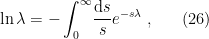
 ![\displaystyle q_\phi(z|x)=\frac{1}{Z_q}e^{-\beta E_q}~, \quad\quad Z_q[\phi]=\sum_ze^{-\beta E_q(x,z;\phi)}~, \ \ \ \ \ (26)](https://s0.wp.com/latex.php?latex=%5Cdisplaystyle+q_%5Cphi%28z%7Cx%29%3D%5Cfrac%7B1%7D%7BZ_q%7De%5E%7B-%5Cbeta+E_q%7D%7E%2C+%5Cquad%5Cquad+Z_q%5B%5Cphi%5D%3D%5Csum_ze%5E%7B-%5Cbeta+E_q%28x%2Cz%3B%5Cphi%29%7D%7E%2C+%5C+%5C+%5C+%5C+%5C+%2826%29&bg=ffffff&fg=000000&s=0&c=20201002)
 , to avoid confusion with
 ![\displaystyle \begin{aligned} F_q[\theta,\phi]&=\sum_z q_\phi(x|z)E_p-\beta^{-1}\sum_z q_\phi(x|z)\left[\beta E_q+\ln Z_q\right]\\ &=\langle E_p(\theta)-E_q(\phi)\rangle_q-\beta^{-1}\ln Z_q[\phi]~. \end{aligned} \ \ \ \ \ (27)](https://s0.wp.com/latex.php?latex=%5Cdisplaystyle+%5Cbegin%7Baligned%7D+F_q%5B%5Ctheta%2C%5Cphi%5D%26%3D%5Csum_z+q_%5Cphi%28x%7Cz%29E_p-%5Cbeta%5E%7B-1%7D%5Csum_z+q_%5Cphi%28x%7Cz%29%5Cleft%5B%5Cbeta+E_q%2B%5Cln+Z_q%5Cright%5D%5C%5C+%26%3D%5Clangle+E_p%28%5Ctheta%29-E_q%28%5Cphi%29%5Crangle_q-%5Cbeta%5E%7B-1%7D%5Cln+Z_q%5B%5Cphi%5D%7E.+%5Cend%7Baligned%7D+%5C+%5C+%5C+%5C+%5C+%2827%29&bg=ffffff&fg=000000&s=0&c=20201002)
 , and similarly for
 ![\displaystyle F_q[\theta,\phi]=\beta^{-1}\sum_z q_\phi(z|x)\ln\frac{q_\phi(z|x)}{p_\theta(z|x)}-\beta^{-1}\ln Z_p[\theta]~, \ \ \ \ \ (28)](https://s0.wp.com/latex.php?latex=%5Cdisplaystyle+F_q%5B%5Ctheta%2C%5Cphi%5D%3D%5Cbeta%5E%7B-1%7D%5Csum_z+q_%5Cphi%28z%7Cx%29%5Cln%5Cfrac%7Bq_%5Cphi%28z%7Cx%29%7D%7Bp_%5Ctheta%28z%7Cx%29%7D-%5Cbeta%5E%7B-1%7D%5Cln+Z_p%5B%5Ctheta%5D%7E%2C+%5C+%5C+%5C+%5C+%5C+%2828%29&bg=ffffff&fg=000000&s=0&c=20201002)
 terms have canceled. Recognizing (5) and (21) on the right-hand side, we therefore find that the difference between the variational and Helmholtz free energies is none other than the KL divergence,
 ![\displaystyle F_q[\theta,\phi]-F_p[\theta]=\beta^{-1}D_z\left(q_\phi(z|x)\,||\,p_\theta(z|x)\right)\geq0~, \ \ \ \ \ (29)](https://s0.wp.com/latex.php?latex=%5Cdisplaystyle+F_q%5B%5Ctheta%2C%5Cphi%5D-F_p%5B%5Ctheta%5D%3D%5Cbeta%5E%7B-1%7DD_z%5Cleft%28q_%5Cphi%28z%7Cx%29%5C%2C%7C%7C%5C%2Cp_%5Ctheta%28z%7Cx%29%5Cright%29%5Cgeq0%7E%2C+%5C+%5C+%5C+%5C+%5C+%2829%29&bg=ffffff&fg=000000&s=0&c=20201002)

 in
in  -dimensional Euclidean spacetime, where
  with
with  . The Euclidean time
  is related to Minkowski time
  via the usual Wick rotation, and we have singled-out one of the transverse coordinates
  ) half of Euclidean spacetime with the boundary condition
  :
:![\displaystyle \Psi[\psi_0(x)]=\int_{\psi(0,x,z)=\psi_0(x,z)}\!\mathcal{D}\psi\,e^{-W[\psi]}~, \ \ \ \ \ (1)](https://s0.wp.com/latex.php?latex=%5Cdisplaystyle+%5CPsi%5B%5Cpsi_0%28x%29%5D%3D%5Cint_%7B%5Cpsi%280%2Cx%2Cz%29%3D%5Cpsi_0%28x%2Cz%29%7D%5C%21%5Cmathcal%7BD%7D%5Cpsi%5C%2Ce%5E%7B-W%5B%5Cpsi%5D%7D%7E%2C+%5C+%5C+%5C+%5C+%5C+%281%29&bg=ffffff&fg=000000&s=0&c=20201002)
 to denote the Euclidean action for the matter field, so as to reserve
  for the entropy.
 surface into two halves,
  and
and  , by defining a codimension-2 surface
  by the condition
  ,
, 
 . In the Euclidean path integral, this corresponds to integrating out
  surface (i.e., along
  as this cut is approached from above (
 ) and below (
 ). Hence:
 ![\displaystyle \rho(\psi_+^1,\psi_+^2)=\int\!\mathcal{D}\psi_-\Psi[\psi_+^1,\psi_-]\Psi[\psi_+^2,\psi_-]~. \ \ \ \ \ (3)](https://s0.wp.com/latex.php?latex=%5Cdisplaystyle+%5Crho%28%5Cpsi_%2B%5E1%2C%5Cpsi_%2B%5E2%29%3D%5Cint%5C%21%5Cmathcal%7BD%7D%5Cpsi_-%5CPsi%5B%5Cpsi_%2B%5E1%2C%5Cpsi_-%5D%5CPsi%5B%5Cpsi_%2B%5E2%2C%5Cpsi_-%5D%7E.+%5C+%5C+%5C+%5C+%5C+%283%29&bg=ffffff&fg=000000&s=0&c=20201002)
 are computed by performing the path integral with the specified boundary conditions along the cut.
 is an impossible task for all but the very simplest systems. Enter the replica trick. The basic idea is to consider the
  subspace in polar coordinates
  , where
  and
and  , such that the cut corresponds to
  for
for  . In constructing the
  to
to  . The resulting space is technically a cone, denoted
  , with angular deficit
  at
at ![\displaystyle Z[C_n]=\mathrm{tr}\rho^n~, \ \ \ \ \ (4)](https://s0.wp.com/latex.php?latex=%5Cdisplaystyle+Z%5BC_n%5D%3D%5Cmathrm%7Btr%7D%5Crho%5En%7E%2C+%5C+%5C+%5C+%5C+%5C+%284%29&bg=ffffff&fg=000000&s=0&c=20201002)
 is the
  power of the density matrix (3). At this point in our
 . Equivalently, we may express the von Neumann entropy directly as
![\displaystyle -(n\partial_n-1)\ln\mathrm{tr}\,\rho^n\big|_{n=1} =-\left[\frac{n}{\mathrm{tr}\rho^n}\,\mathrm{tr}\!\left(\rho^n\ln\rho\right)-\ln\mathrm{tr}\rho^n\right]\bigg|_{n=1} =-\mathrm{tr}\left(\rho\ln\rho\right)~, \ \ \ \ \ (7)](https://s0.wp.com/latex.php?latex=%5Cdisplaystyle+-%28n%5Cpartial_n-1%29%5Cln%5Cmathrm%7Btr%7D%5C%2C%5Crho%5En%5Cbig%7C_%7Bn%3D1%7D+%3D-%5Cleft%5B%5Cfrac%7Bn%7D%7B%5Cmathrm%7Btr%7D%5Crho%5En%7D%5C%2C%5Cmathrm%7Btr%7D%5C%21%5Cleft%28%5Crho%5En%5Cln%5Crho%5Cright%29-%5Cln%5Cmathrm%7Btr%7D%5Crho%5En%5Cright%5D%5Cbigg%7C_%7Bn%3D1%7D+%3D-%5Cmathrm%7Btr%7D%5Cleft%28%5Crho%5Cln%5Crho%5Cright%29%7E%2C+%5C+%5C+%5C+%5C+%5C+%287%29&bg=ffffff&fg=000000&s=0&c=20201002)
 , whereupon the second term vanishes. Et voilà! As I understand it, the aforementioned “conical singularity method” is essentially an abstraction of the replica trick to spacetimes with conical singularities. Hence, re-purposing our notation, consider the effective action
 ![{W[\alpha]=-\ln Z[C_\alpha]}](https://s0.wp.com/latex.php?latex=%7BW%5B%5Calpha%5D%3D-%5Cln+Z%5BC_%5Calpha%5D%7D&bg=ffffff&fg=000000&s=0&c=20201002) for fields on a Euclidean spacetime with a conical singularity at
for fields on a Euclidean spacetime with a conical singularity at  is defined, in polar coordinates, by making
  , and taking the limit in which the deficit
  . The entanglement entropy for fields on this background is then
 ![\displaystyle S=(\alpha\partial_\alpha-1)W[\alpha]\big|_{\alpha=1}~. \ \ \ \ \ (8)](https://s0.wp.com/latex.php?latex=%5Cdisplaystyle+S%3D%28%5Calpha%5Cpartial_%5Calpha-1%29W%5B%5Calpha%5D%5Cbig%7C_%7B%5Calpha%3D1%7D%7E.+%5C+%5C+%5C+%5C+%5C+%288%29&bg=ffffff&fg=000000&s=0&c=20201002)
 to non-integer values. We’ve discussed this issue
  , where
  is an arbitrary constant. This is actually an important constraint to bear in mind when attempting to infer general physical lessons from our results, but we’ll address this caveat later. Suffice to say that given this assumption, the analytical continuation can be uniquely performed without obstruction; see in particular section 2.7 of [1] for details.
 of a kernel satisfying the heat equation. This enables one to express the effective action as
 is the (trace of the) heat kernel for the Laplacian operator
  acting on distributions with support on
  . If
. If  admits a right inverse, then the latter defines the Green function
  as the solution to the inhomogeneous differential equation
 represent vectors in

 and integrate w.r.t
  ; by virtue of the delta function (and the fact that
 then determine the precise form of
  (e.g.,
  for a scalar field
  is a Green function for the Klein-Gordon operator, since it satisfies the equation


 . In the second equality, we’ve written the operator in the so-called canonical form for a Laplacian operator on a vector bundle, where
  is an endomorphism on the bundle over the manifold, and the covariant derivative
  includes both the familiar Riemann part as well as the contribution from the gauge (bundle) part; the field strength for the latter will be denoted
  . Fibre bundles won’t be terribly important for our purposes, but we’ll need some of this notation later; see section 2.1 of [2] for details.
 , the right-hand side of (17) would correspond to the transition amplitude
  for some unitary operator

 is meant to emphasize the fact that the operator
![\displaystyle Z[J]=\int\!\mathcal{D}\psi\,e^{-W[\psi,J]}~, \ \ \ \ \ (22)](https://s0.wp.com/latex.php?latex=%5Cdisplaystyle+Z%5BJ%5D%3D%5Cint%5C%21%5Cmathcal%7BD%7D%5Cpsi%5C%2Ce%5E%7B-W%5B%5Cpsi%2CJ%5D%7D%7E%2C+%5C+%5C+%5C+%5C+%5C+%2822%29&bg=ffffff&fg=000000&s=0&c=20201002)
 is the source for the matter field
  . The heat kernel method applies to one-loop calculations, in which case it suffices to expand the action to quadratic order in fluctuations around the classical saddle-point
  , whence the Gaussian integral may be written
![\displaystyle Z[J]=e^{-S_\mathrm{cl}}\,\mathrm{det}^{-1/2}(D)\,\mathrm{exp}\left(\frac{1}{4}JD^{-1}J\right)~. \ \ \ \ \ (23)](https://s0.wp.com/latex.php?latex=%5Cdisplaystyle+Z%5BJ%5D%3De%5E%7B-S_%5Cmathrm%7Bcl%7D%7D%5C%2C%5Cmathrm%7Bdet%7D%5E%7B-1%2F2%7D%28D%29%5C%2C%5Cmathrm%7Bexp%7D%5Cleft%28%5Cfrac%7B1%7D%7B4%7DJD%5E%7B-1%7DJ%5Cright%29%7E.+%5C+%5C+%5C+%5C+%5C+%2823%29&bg=ffffff&fg=000000&s=0&c=20201002)
 , thereby identifying it with the two-point correlator for
 ![\displaystyle G(x,y)=\langle\psi(x)\psi(y)\rangle=\frac{1}{Z[0]}\left.\frac{\delta^2 Z[J]}{\delta J(x)\delta J(y)}\right|_{J=0}=D^{-1}~, \ \ \ \ \ (24)](https://s0.wp.com/latex.php?latex=%5Cdisplaystyle+G%28x%2Cy%29%3D%5Clangle%5Cpsi%28x%29%5Cpsi%28y%29%5Crangle%3D%5Cfrac%7B1%7D%7BZ%5B0%5D%7D%5Cleft.%5Cfrac%7B%5Cdelta%5E2+Z%5BJ%5D%7D%7B%5Cdelta+J%28x%29%5Cdelta+J%28y%29%7D%5Cright%7C_%7BJ%3D0%7D%3DD%5E%7B-1%7D%7E%2C+%5C+%5C+%5C+%5C+%5C+%2824%29&bg=ffffff&fg=000000&s=0&c=20201002)
 (strictly speaking, this identity is only correct up to a constant, but we may normalize away this inconvenience anyway; did I mention I’d be somewhat cavalier?). We then apply this identity to every (positive) eigenvalue
  of
of 


 — an asymptotic series gives finite results for fixed
  . Second, we are ignoring various subtleties regarding the rigorous definition of the trace, wherein both (29) and (28) are properly defined via the use of an auxiliary function; cf. eq. (2.21) of [2] (n.b., Vassilevich’s coefficients do not include the normalization
  from the volume integrals; see below).
 is that they can be expressed as integrals of local invariants—tensor quantities which remain invariant under local diffeomorphisms; e.g., the Riemann curvature tensor and covariant derivatives thereof. Thus the first step in the procedure for calculating the heat kernel coefficients is to write down the integral over all such local invariants; for example, the first three coefficients are
 were introduced in (18). A word of warning, for those of you cross-referencing with Solodukhin [1] and Vassilevich [2]: these coefficients correspond to eqs. (4.13) – (4.15) in [2], except that we have already included the normalization
  . This is a rather involved technical procedure, but is explained in detail in section 4.1 of [2]. One finds
![\displaystyle \begin{aligned} a_0(D)&=\int_M1~,\\ a_1(D)&=\int_M\left(E+\tfrac{1}{6}R\right)~,\\ a_2(D)&=\int_M\left[\tfrac{1}{180}R_{ijkl}^2-\tfrac{1}{180}R_{ij}^2+\tfrac{1}{6}\nabla^2\left(E+\tfrac{1}{5}R\right)+\tfrac{1}{2}\left(E+\tfrac{1}{6}R\right)^2\right]~, \end{aligned} \ \ \ \ \ (32)](https://s0.wp.com/latex.php?latex=%5Cdisplaystyle+%5Cbegin%7Baligned%7D+a_0%28D%29%26%3D%5Cint_M1%7E%2C%5C%5C+a_1%28D%29%26%3D%5Cint_M%5Cleft%28E%2B%5Ctfrac%7B1%7D%7B6%7DR%5Cright%29%7E%2C%5C%5C+a_2%28D%29%26%3D%5Cint_M%5Cleft%5B%5Ctfrac%7B1%7D%7B180%7DR_%7Bijkl%7D%5E2-%5Ctfrac%7B1%7D%7B180%7DR_%7Bij%7D%5E2%2B%5Ctfrac%7B1%7D%7B6%7D%5Cnabla%5E2%5Cleft%28E%2B%5Ctfrac%7B1%7D%7B5%7DR%5Cright%29%2B%5Ctfrac%7B1%7D%7B2%7D%5Cleft%28E%2B%5Ctfrac%7B1%7D%7B6%7DR%5Cright%29%5E2%5Cright%5D%7E%2C+%5Cend%7Baligned%7D+%5C+%5C+%5C+%5C+%5C+%2832%29&bg=ffffff&fg=000000&s=0&c=20201002)
 ; we have also set the gauge field strength
  for simplicity, since we will consider only free scalar fields below. These correspond to what Solodukhin refers to as regular coefficients, cf. his eq. (69). If one is working on a background with conical singularities, then there are additional contributions from the singular surface
 and
and  , where
  are orthonormal vectors orthogonal to
  in (32) is the
  , and are related to their flat counterparts by eq. (55) of [1]. Of course, here and in (33),
  , not to be confused with the constants
  , where
  , on some background spacetime
  in
in  dimensions, with a conical deficit at the codimension-2 surface
  -dimensional surface may be calculated directly from the coefficient
  above. To this order in the expansion, the relevant part of
 ![\displaystyle \begin{aligned} W[\alpha]&\simeq-\frac{1}{2}\int_{\epsilon^2}^\infty\!\frac{\mathrm{d} s}{s}(4\pi s)^{-d/2}\left(a_0^\Sigma+a_1^\Sigma s\right) =-\frac{\pi}{6}\frac{(1-\alpha)(1+\alpha)}{\alpha}\int_{\epsilon^2}^{\infty}\!\frac{\mathrm{d} s}{(4\pi s)^{d/2}}\int_\Sigma1\\ &=\frac{-1}{12(d\!-\!2)(4\pi)^{(d-2)/2}}\frac{A(\Sigma)}{\epsilon^{d-2}}\frac{(1-\alpha)(1+\alpha)}{\alpha}~, \end{aligned} \ \ \ \ \ (34)](https://s0.wp.com/latex.php?latex=%5Cdisplaystyle+%5Cbegin%7Baligned%7D+W%5B%5Calpha%5D%26%5Csimeq-%5Cfrac%7B1%7D%7B2%7D%5Cint_%7B%5Cepsilon%5E2%7D%5E%5Cinfty%5C%21%5Cfrac%7B%5Cmathrm%7Bd%7D+s%7D%7Bs%7D%284%5Cpi+s%29%5E%7B-d%2F2%7D%5Cleft%28a_0%5E%5CSigma%2Ba_1%5E%5CSigma+s%5Cright%29+%3D-%5Cfrac%7B%5Cpi%7D%7B6%7D%5Cfrac%7B%281-%5Calpha%29%281%2B%5Calpha%29%7D%7B%5Calpha%7D%5Cint_%7B%5Cepsilon%5E2%7D%5E%7B%5Cinfty%7D%5C%21%5Cfrac%7B%5Cmathrm%7Bd%7D+s%7D%7B%284%5Cpi+s%29%5E%7Bd%2F2%7D%7D%5Cint_%5CSigma1%5C%5C+%26%3D%5Cfrac%7B-1%7D%7B12%28d%5C%21-%5C%212%29%284%5Cpi%29%5E%7B%28d-2%29%2F2%7D%7D%5Cfrac%7BA%28%5CSigma%29%7D%7B%5Cepsilon%5E%7Bd-2%7D%7D%5Cfrac%7B%281-%5Calpha%29%281%2B%5Calpha%29%7D%7B%5Calpha%7D%7E%2C+%5Cend%7Baligned%7D+%5C+%5C+%5C+%5C+%5C+%2834%29&bg=ffffff&fg=000000&s=0&c=20201002)
 in the lower limit of integration, to make the dimensions of the auxiliary time variable work-out; this is perhaps clearest by examining eq. (1.12) of [2]) and the area of the surface
  . Substituting this expression for the effective action into eq. (8) for the entropy, we obtain

 we also have a log divergence from the
  term:
term:![\displaystyle \begin{aligned} W[\alpha]&=-\frac{1}{2}\int_{\epsilon^2}^\infty\!\frac{\mathrm{d} s}{s}(4\pi s)^{-d/2}\left(a_0^\Sigma+a_1^\Sigma s+a_2^\Sigma s^2+\ldots\right)\\ &=-\frac{1}{32\pi^2}\int_{\epsilon^2}^\infty\!\mathrm{d} s\left(\frac{a_1^\Sigma}{s^2}+\frac{a_2^\Sigma}{s}+O(s^0)\right) \simeq-\frac{1}{32\pi^2}\left(\frac{a_1^\Sigma}{\epsilon^2}-2a_2^\Sigma\ln\epsilon\right)~, \end{aligned} \ \ \ \ \ (37)](https://s0.wp.com/latex.php?latex=%5Cdisplaystyle+%5Cbegin%7Baligned%7D+W%5B%5Calpha%5D%26%3D-%5Cfrac%7B1%7D%7B2%7D%5Cint_%7B%5Cepsilon%5E2%7D%5E%5Cinfty%5C%21%5Cfrac%7B%5Cmathrm%7Bd%7D+s%7D%7Bs%7D%284%5Cpi+s%29%5E%7B-d%2F2%7D%5Cleft%28a_0%5E%5CSigma%2Ba_1%5E%5CSigma+s%2Ba_2%5E%5CSigma+s%5E2%2B%5Cldots%5Cright%29%5C%5C+%26%3D-%5Cfrac%7B1%7D%7B32%5Cpi%5E2%7D%5Cint_%7B%5Cepsilon%5E2%7D%5E%5Cinfty%5C%21%5Cmathrm%7Bd%7D+s%5Cleft%28%5Cfrac%7Ba_1%5E%5CSigma%7D%7Bs%5E2%7D%2B%5Cfrac%7Ba_2%5E%5CSigma%7D%7Bs%7D%2BO%28s%5E0%29%5Cright%29+%5Csimeq-%5Cfrac%7B1%7D%7B32%5Cpi%5E2%7D%5Cleft%28%5Cfrac%7Ba_1%5E%5CSigma%7D%7B%5Cepsilon%5E2%7D-2a_2%5E%5CSigma%5Cln%5Cepsilon%5Cright%29%7E%2C+%5Cend%7Baligned%7D+%5C+%5C+%5C+%5C+%5C+%2837%29&bg=ffffff&fg=000000&s=0&c=20201002)
 term results in an expression for the UV divergent part of the black hole entanglement entropy of the form
![\displaystyle S_\mathrm{ent}=\frac{A(\sigma)}{48\pi\epsilon^2} -\frac{1}{144\pi}\int_\Sigma\left[6E+R-\frac{1}{5}\left(R_{ii}-2R_{ijij}\right)\right]\ln\epsilon~, \ \ \ \ \ (38)](https://s0.wp.com/latex.php?latex=%5Cdisplaystyle+S_%5Cmathrm%7Bent%7D%3D%5Cfrac%7BA%28%5Csigma%29%7D%7B48%5Cpi%5Cepsilon%5E2%7D+-%5Cfrac%7B1%7D%7B144%5Cpi%7D%5Cint_%5CSigma%5Cleft%5B6E%2BR-%5Cfrac%7B1%7D%7B5%7D%5Cleft%28R_%7Bii%7D-2R_%7Bijij%7D%5Cright%29%5Cright%5D%5Cln%5Cepsilon%7E%2C+%5C+%5C+%5C+%5C+%5C+%2838%29&bg=ffffff&fg=000000&s=0&c=20201002)
 and
and  , respectively). For the simplest case of a massless, minimally coupled scalar field (
 ) on a Schwarzschild black hole background, the above yields
 is the horizon radius; see section 3.9.1 of [1] for more details. Note that since the Ricci scalar
  , the logarithmic term represents a purely topological correction to the flat space entropy (36) (in contrast to flat space, the Euler number for a black hole geometry is non-zero). Curvature corrections can still show up in UV-finite terms, of course, but that’s not what we’re seeing here: in this sense the log term is universal.
![{F=\beta^{-1}\ln Z[\beta,g]}](https://s0.wp.com/latex.php?latex=%7BF%3D%5Cbeta%5E%7B-1%7D%5Cln+Z%5B%5Cbeta%2Cg%5D%7D&bg=ffffff&fg=000000&s=0&c=20201002) w.r.t. temperature
w.r.t. temperature ![\displaystyle S_\mathrm{thermo}=\frac{\mathrm{d} F}{\mathrm{d} T}=-\beta^2\frac{\mathrm{d} F}{\mathrm{d} \beta} =\left(\beta\frac{\mathrm{d}}{\mathrm{d}\beta}-1\right)W_\mathrm{tot}[\beta,g]~, \ \ \ \ \ (40)](https://s0.wp.com/latex.php?latex=%5Cdisplaystyle+S_%5Cmathrm%7Bthermo%7D%3D%5Cfrac%7B%5Cmathrm%7Bd%7D+F%7D%7B%5Cmathrm%7Bd%7D+T%7D%3D-%5Cbeta%5E2%5Cfrac%7B%5Cmathrm%7Bd%7D+F%7D%7B%5Cmathrm%7Bd%7D+%5Cbeta%7D+%3D%5Cleft%28%5Cbeta%5Cfrac%7B%5Cmathrm%7Bd%7D%7D%7B%5Cmathrm%7Bd%7D%5Cbeta%7D-1%5Cright%29W_%5Cmathrm%7Btot%7D%5B%5Cbeta%2Cg%5D%7E%2C+%5C+%5C+%5C+%5C+%5C+%2840%29&bg=ffffff&fg=000000&s=0&c=20201002)
![{W_\mathrm{tot}[\beta,g]=\ln Z[\beta,g]}](https://s0.wp.com/latex.php?latex=%7BW_%5Cmathrm%7Btot%7D%5B%5Cbeta%2Cg%5D%3D%5Cln+Z%5B%5Cbeta%2Cg%5D%7D&bg=ffffff&fg=000000&s=0&c=20201002) . Crucially, observe that here, in contrast to our partition function (22) for fields on a fixed background, the total Euclidean path integral that prepares the state also includes an integration over the metrics:
. Crucially, observe that here, in contrast to our partition function (22) for fields on a fixed background, the total Euclidean path integral that prepares the state also includes an integration over the metrics: ![\displaystyle Z[\beta,g]=\int\!\mathcal{D} g_{\mu\nu}\,\mathcal{D}\psi\,e^{-W_\mathrm{gr}[g]+W_\mathrm{mat}[\psi,g]}~, \ \ \ \ \ (41)](https://s0.wp.com/latex.php?latex=%5Cdisplaystyle+Z%5B%5Cbeta%2Cg%5D%3D%5Cint%5C%21%5Cmathcal%7BD%7D+g_%7B%5Cmu%5Cnu%7D%5C%2C%5Cmathcal%7BD%7D%5Cpsi%5C%2Ce%5E%7B-W_%5Cmathrm%7Bgr%7D%5Bg%5D%2BW_%5Cmathrm%7Bmat%7D%5B%5Cpsi%2Cg%5D%7D%7E%2C+%5C+%5C+%5C+%5C+%5C+%2841%29&bg=ffffff&fg=000000&s=0&c=20201002)
 represents the gravitational part of the action (e.g., the Einstein-Hilbert term), and
  the contribution from the matter fields. (For reference, we’re following the reasoning and notation in section 4.1 of [1] here).
 in the highly symmetric case of Schwarzschild, and suitable asymptotic behaviour at large radius. Hence in computing this path integral, one first performs the integration over matter fields
 ![\displaystyle \int\!\mathcal{D}\psi\,e^{-W_\mathrm{mat}[\psi,g]}=e^{-W[\beta,g]}~, \ \ \ \ \ (42)](https://s0.wp.com/latex.php?latex=%5Cdisplaystyle+%5Cint%5C%21%5Cmathcal%7BD%7D%5Cpsi%5C%2Ce%5E%7B-W_%5Cmathrm%7Bmat%7D%5B%5Cpsi%2Cg%5D%7D%3De%5E%7B-W%5B%5Cbeta%2Cg%5D%7D%7E%2C+%5C+%5C+%5C+%5C+%5C+%2842%29&bg=ffffff&fg=000000&s=0&c=20201002)
![{W[\beta,g]}](https://s0.wp.com/latex.php?latex=%7BW%5B%5Cbeta%2Cg%5D%7D&bg=ffffff&fg=000000&s=0&c=20201002) represents the effective action for the fields described above; note that the contribution from entanglement entropy is entirely encoded in this portion. The path integral (41) now looks like this:
represents the effective action for the fields described above; note that the contribution from entanglement entropy is entirely encoded in this portion. The path integral (41) now looks like this:![\displaystyle Z[\beta,g]=\int\!\mathcal{D} g\,e^{-W_\mathrm{gr}[\psi,g]-W[\beta,g]} \simeq e^{-W_\mathrm{tot}[\beta,\,g(\beta)]}~, \ \ \ \ \ (43)](https://s0.wp.com/latex.php?latex=%5Cdisplaystyle+Z%5B%5Cbeta%2Cg%5D%3D%5Cint%5C%21%5Cmathcal%7BD%7D+g%5C%2Ce%5E%7B-W_%5Cmathrm%7Bgr%7D%5B%5Cpsi%2Cg%5D-W%5B%5Cbeta%2Cg%5D%7D+%5Csimeq+e%5E%7B-W_%5Cmathrm%7Btot%7D%5B%5Cbeta%2C%5C%2Cg%28%5Cbeta%29%5D%7D%7E%2C+%5C+%5C+%5C+%5C+%5C+%2843%29&bg=ffffff&fg=000000&s=0&c=20201002)
 on the far right is the semiclassical effective action obtained from the saddle-point approximation. That is, the metric
  is the solution to
 ![\displaystyle \frac{\delta W_\mathrm{tot}[\beta,g]}{\delta g}=0~, \qquad\mathrm{with}\qquad W_\mathrm{tot}=W_\mathrm{gr}+W \ \ \ \ \ (44)](https://s0.wp.com/latex.php?latex=%5Cdisplaystyle+%5Cfrac%7B%5Cdelta+W_%5Cmathrm%7Btot%7D%5B%5Cbeta%2Cg%5D%7D%7B%5Cdelta+g%7D%3D0%7E%2C+%5Cqquad%5Cmathrm%7Bwith%7D%5Cqquad+W_%5Cmathrm%7Btot%7D%3DW_%5Cmathrm%7Bgr%7D%2BW+%5C+%5C+%5C+%5C+%5C+%2844%29&bg=ffffff&fg=000000&s=0&c=20201002)
 fluctuates due to the quantum corrections represented by the second term
 ![\displaystyle S_\mathrm{thermo}= \beta\left(\partial_\beta W_\mathrm{tot}[\beta,g]+\frac{\delta g_{\mu\nu}(\beta)}{\delta\beta}\frac{\delta W_\mathrm{tot}[\beta,g]}{\delta g_{\mu\nu}(\beta)}\right) -W_\mathrm{tot}[\beta,g]~, \ \ \ \ \ (45)](https://s0.wp.com/latex.php?latex=%5Cdisplaystyle+S_%5Cmathrm%7Bthermo%7D%3D+%5Cbeta%5Cleft%28%5Cpartial_%5Cbeta+W_%5Cmathrm%7Btot%7D%5B%5Cbeta%2Cg%5D%2B%5Cfrac%7B%5Cdelta+g_%7B%5Cmu%5Cnu%7D%28%5Cbeta%29%7D%7B%5Cdelta%5Cbeta%7D%5Cfrac%7B%5Cdelta+W_%5Cmathrm%7Btot%7D%5B%5Cbeta%2Cg%5D%7D%7B%5Cdelta+g_%7B%5Cmu%5Cnu%7D%28%5Cbeta%29%7D%5Cright%29+-W_%5Cmathrm%7Btot%7D%5B%5Cbeta%2Cg%5D%7E%2C+%5C+%5C+%5C+%5C+%5C+%2845%29&bg=ffffff&fg=000000&s=0&c=20201002)
![\displaystyle S_\mathrm{thermo}=\left(\beta\partial_\beta-1\right)W_\mathrm{tot}[\beta,g] =\left(\beta\partial_\beta-1\right)\left(W_\mathrm{gr}+W\right) =S_\mathrm{gr}+S_\mathrm{ent}~. \ \ \ \ \ (46)](https://s0.wp.com/latex.php?latex=%5Cdisplaystyle+S_%5Cmathrm%7Bthermo%7D%3D%5Cleft%28%5Cbeta%5Cpartial_%5Cbeta-1%5Cright%29W_%5Cmathrm%7Btot%7D%5B%5Cbeta%2Cg%5D+%3D%5Cleft%28%5Cbeta%5Cpartial_%5Cbeta-1%5Cright%29%5Cleft%28W_%5Cmathrm%7Bgr%7D%2BW%5Cright%29+%3DS_%5Cmathrm%7Bgr%7D%2BS_%5Cmathrm%7Bent%7D%7E.+%5C+%5C+%5C+%5C+%5C+%2846%29&bg=ffffff&fg=000000&s=0&c=20201002)
 is a statement about the possible internal microstates at equilibrium — meaning, states which satisfy the quantum-corrected Einstein equations (44) — which therefore includes the entropy from possible (regular) metric configurations
  as well as the quantum corrections
  given by (39).
 refers only to the gravitational entropy, i.e.,
  . This is sometimes referred to as the “classical” part, because it represents the tree-level contribution to the path integral result. That is, if we were to restore Planck’s constant, we’d find that
  prefactor, while
  . Accordingly,
  -expansion.)
![\displaystyle e^{\frac{1}{2}\sum_{ij}K_{ij}s_is_j} =\left[\frac{\mathrm{det}K}{(2\pi)^N}\right]^{1/2}\prod_{k=1}^N\int\!\mathrm{d}\phi_k\exp\left(-\frac{1}{2}\sum_{ij}K_{ij}\phi_i\phi_j+\sum_{ij}K_{ij}s_i\phi_j\right)~, \ \ \ \ \ (2)](https://s0.wp.com/latex.php?latex=%5Cdisplaystyle+e%5E%7B%5Cfrac%7B1%7D%7B2%7D%5Csum_%7Bij%7DK_%7Bij%7Ds_is_j%7D+%3D%5Cleft%5B%5Cfrac%7B%5Cmathrm%7Bdet%7DK%7D%7B%282%5Cpi%29%5EN%7D%5Cright%5D%5E%7B1%2F2%7D%5Cprod_%7Bk%3D1%7D%5EN%5Cint%5C%21%5Cmathrm%7Bd%7D%5Cphi_k%5Cexp%5Cleft%28-%5Cfrac%7B1%7D%7B2%7D%5Csum_%7Bij%7DK_%7Bij%7D%5Cphi_i%5Cphi_j%2B%5Csum_%7Bij%7DK_%7Bij%7Ds_i%5Cphi_j%5Cright%29%7E%2C+%5C+%5C+%5C+%5C+%5C+%282%29&bg=ffffff&fg=000000&s=0&c=20201002)
 is the total number of spins. Now consider the Ising model with nearest-neighbor interactions, whose hamiltonian is
 , and symmetric coupling matrix
  if
if  are nearest-neighbors, and zero otherwise. The partition function is
![\displaystyle \begin{aligned} {}&\sum_{s_i=\pm1}\exp\left(\sum\nolimits_{ij}K_{ij}s_i\phi_j\right) =\sum_{s_i=\pm1}\prod_i\exp\left(\sum\nolimits_{j}K_{ij}s_i\phi_j\right)\\ &=\prod_i\left[\exp\left(\sum\nolimits_{j}K_{ij}\phi_j\right)+\exp\left(-\sum\nolimits_{j}K_{ij}\phi_j\right)\right]\\ &=2^N\prod_i\cosh\left(\sum\nolimits_{j}K_{ij}\phi_j\right) =2^N\exp\left[\sum\nolimits_i\ln\cosh\left(\sum\nolimits_jK_{ij}\phi_j\right)\right]~, \end{aligned} \ \ \ \ \ (5)](https://s0.wp.com/latex.php?latex=%5Cdisplaystyle+%5Cbegin%7Baligned%7D+%7B%7D%26%5Csum_%7Bs_i%3D%5Cpm1%7D%5Cexp%5Cleft%28%5Csum%5Cnolimits_%7Bij%7DK_%7Bij%7Ds_i%5Cphi_j%5Cright%29+%3D%5Csum_%7Bs_i%3D%5Cpm1%7D%5Cprod_i%5Cexp%5Cleft%28%5Csum%5Cnolimits_%7Bj%7DK_%7Bij%7Ds_i%5Cphi_j%5Cright%29%5C%5C+%26%3D%5Cprod_i%5Cleft%5B%5Cexp%5Cleft%28%5Csum%5Cnolimits_%7Bj%7DK_%7Bij%7D%5Cphi_j%5Cright%29%2B%5Cexp%5Cleft%28-%5Csum%5Cnolimits_%7Bj%7DK_%7Bij%7D%5Cphi_j%5Cright%29%5Cright%5D%5C%5C+%26%3D2%5EN%5Cprod_i%5Ccosh%5Cleft%28%5Csum%5Cnolimits_%7Bj%7DK_%7Bij%7D%5Cphi_j%5Cright%29+%3D2%5EN%5Cexp%5Cleft%5B%5Csum%5Cnolimits_i%5Cln%5Ccosh%5Cleft%28%5Csum%5Cnolimits_jK_%7Bij%7D%5Cphi_j%5Cright%29%5Cright%5D%7E%2C+%5Cend%7Baligned%7D+%5C+%5C+%5C+%5C+%5C+%285%29&bg=ffffff&fg=000000&s=0&c=20201002)
![\displaystyle Z=\left[\frac{\mathrm{det}K}{(\pi/2)^N}\right]^{1/2}\prod_{k=1}^N\int\!\mathrm{d}\phi_k\exp\left(-\frac{1}{2}\sum_{ij}K_{ij}\phi_i\phi_j+\sum\nolimits_i\ln\cosh\sum\nolimits_jK_{ij}\phi_j\right)~, \ \ \ \ \ (6)](https://s0.wp.com/latex.php?latex=%5Cdisplaystyle+Z%3D%5Cleft%5B%5Cfrac%7B%5Cmathrm%7Bdet%7DK%7D%7B%28%5Cpi%2F2%29%5EN%7D%5Cright%5D%5E%7B1%2F2%7D%5Cprod_%7Bk%3D1%7D%5EN%5Cint%5C%21%5Cmathrm%7Bd%7D%5Cphi_k%5Cexp%5Cleft%28-%5Cfrac%7B1%7D%7B2%7D%5Csum_%7Bij%7DK_%7Bij%7D%5Cphi_i%5Cphi_j%2B%5Csum%5Cnolimits_i%5Cln%5Ccosh%5Csum%5Cnolimits_jK_%7Bij%7D%5Cphi_j%5Cright%29%7E%2C+%5C+%5C+%5C+%5C+%5C+%286%29&bg=ffffff&fg=000000&s=0&c=20201002)
 . We have thus obtained an exact transformation from the original, discrete model of spins to an equivalent, continuum field theory. To proceed with renormalization of this model, we refer the interested reader to the aforementioned Vvedensky reference. The remarkable upshot, for our purposes, is that all of the physics of the original spin degrees of freedom are entirely encoded in the new field
 is a vector of visible neurons, and on the second line we’ve appealed to SVD to decompose the coupling matrix as
  . In its current form, the visible neurons interact directly through the second, coupling term. We now wish to introduce latent or hidden variables
  that mediate this coupling instead. To do this, consider the Hubbard-Stratonovish transformation
  ,
,  , and
, and  . Then the second term in


 is now mediated via the latent degrees of freedom
  instead. As we’ll see below, this basic mechanism can be readily generalized such that we can encode arbitrarily complex — that is, arbitrarily high-order — interactions between visible neurons by coupling to a second layer of hidden neurons.
 and
and  can be freely chosen. According to Mehta et al., the most common choices are
 . Of course, if we marginalize over (i.e., integrate out) the latent variable
  , we recover the distribution of visible neurons, cf.

 , we follow Mehta et al. in introducing the distribution of hidden neurons, ignoring their interaction with the visible layer:
![\displaystyle K_\mu(t)=\ln E_q\left[e^{th_\mu}\right] =\ln\int\!\mathrm{d} h_\mu\,q_\mu(h_\mu)e^{th_\mu} =\sum_n\kappa_\mu^{(n)}\frac{t^n}{n!}~, \ \ \ \ \ (17)](https://s0.wp.com/latex.php?latex=%5Cdisplaystyle+K_%5Cmu%28t%29%3D%5Cln+E_q%5Cleft%5Be%5E%7Bth_%5Cmu%7D%5Cright%5D+%3D%5Cln%5Cint%5C%21%5Cmathrm%7Bd%7D+h_%5Cmu%5C%2Cq_%5Cmu%28h_%5Cmu%29e%5E%7Bth_%5Cmu%7D+%3D%5Csum_n%5Ckappa_%5Cmu%5E%7B%28n%29%7D%5Cfrac%7Bt%5En%7D%7Bn%21%7D%7E%2C+%5C+%5C+%5C+%5C+%5C+%2817%29&bg=ffffff&fg=000000&s=0&c=20201002)
![{E_q[\cdot]}](https://s0.wp.com/latex.php?latex=%7BE_q%5B%5Ccdot%5D%7D&bg=ffffff&fg=000000&s=0&c=20201002) is the expectation value with respect to the distribution
is the expectation value with respect to the distribution  , and the
  is obtained by differentiating the power series
  , i.e.,
  . The reason for introducing
  are actually encoded in the marginal energy distribution
  in the cumulant generating function yields precisely the log term in
 , the free energy
  likewise generates thermodynamic features of the system via its derivatives. Pursuing this here would take us too far afield, but it’s interesting to note
 is the probability of the
  outcome/microstate. However, as Jaynes rightfully stresses, the fact that these concepts share the same mathematical form does not necessarily imply any relation between them. Nonetheless, a physicist cannot resist the intuitive sense that there must be some deeper relationship lurking beneath the surface. And indeed, Jaynes paper [1] makes it beautifully clear that in fact these distinct notions are referencing the same underlying concept—though I may differ from Jaynes in explaining precisely how the subjective/objective divide is crossed.
 , known as Boltzmann’s constant. This is merely a compensatory factor, to account for humans’ rather arbitrary decision to measure temperatures relative to the freezing point of water at atmospheric pressure. Being civilized people, we shall instead work in natural units, in which
  .)
.) . These could represent, e.g., particular outcomes or measurement values. To each
  , we associated the corresponding probability
  , with
  . The question is then whether one can find a function
  which uniquely quantifies the amount of uncertainty represented by this probability distribution. Remarkably, Shannon showed [2] that this can indeed be done, provided
  satisfies the following three properties:
 (since probabilities sum to 1), and
  is a monotonically increasing function of
  On the left, we have three probabilities
  ,
,  , and
, and  , so the uncertainty for this distribution is given by
  . On the right, we’ve coarse-grained the system such that at the highest level (that is, the left-most branch), we have two equally likely outcomes, and hence uncertainty
  . However, this represents a different state of knowledge than the original
 prefactor is the probabilistic weight associated with this composition of events.
 , which results in the requirement
 , and let
  . If all
  outcomes are equally likely, then the uncertainty, given by the left-hand side of
  . As in the previous example, we want this uncertainty to be preserved under coarse-graining, where in this case we group the possible outcomes into
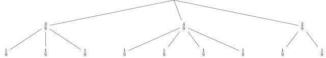
 . The second term on the right-hand side of
  , in which case
  , and
, and  , the solution to which is
  , where
  ). Substituting this into
 . QED.
 ,
, 
 ? As it stands, the problem is insoluble: we need to know
  , but the normalization

 then returns the two constraint equations, along with


 corresponds to the thermodynamic energy, and
  , which may generically depend on other parameters
  ; see [1] for details—Jaynes paper is a gem, and well-worth reading.
 between the
  neurons (with
  ). A neuron is a binary variable which has a value of either 1 (excited) or 0 (quiescent). As the network is evolved in time, the state of the
 is the threshold for the neuron (i.e., a free parameter that determines that neuron’s sensitivity to firing), and in the second equality we have absorbed this by defining the zeroth neuron with
  and
and  . The state of the neuron is updated to 1 with probability
  , and 0 with probability
  , where
 , and hence the transition between states forms a Markov chain with
  sites. In particular, if there are no disconnected nodes, then it forms an ergodic Markov chain with a unique stationary distribution

 as the energy of the state
  , which is given by
 .
. , where
  denotes the state in which the
 ![\displaystyle \begin{aligned} \Delta E&=-\ln p(x_i\!=\!1)+\ln p(x_i\!=\!0) =-\ln p(x_i\!=\!1)+\ln [1-p(x_i\!=\!1)]\\ &=\ln\left[\frac{1}{p(x_i\!=\!1)}-1\right] \;\implies\; p(x_i\!=\!1)=\frac{1}{1+e^{\Delta E}}~, \end{aligned} \ \ \ \ \ (6)](https://s0.wp.com/latex.php?latex=%5Cdisplaystyle+%5Cbegin%7Baligned%7D+%5CDelta+E%26%3D-%5Cln+p%28x_i%5C%21%3D%5C%211%29%2B%5Cln+p%28x_i%5C%21%3D%5C%210%29+%3D-%5Cln+p%28x_i%5C%21%3D%5C%211%29%2B%5Cln+%5B1-p%28x_i%5C%21%3D%5C%211%29%5D%5C%5C+%26%3D%5Cln%5Cleft%5B%5Cfrac%7B1%7D%7Bp%28x_i%5C%21%3D%5C%211%29%7D-1%5Cright%5D+%5C%3B%5Cimplies%5C%3B+p%28x_i%5C%21%3D%5C%211%29%3D%5Cfrac%7B1%7D%7B1%2Be%5E%7B%5CDelta+E%7D%7D%7E%2C+%5Cend%7Baligned%7D+%5C+%5C+%5C+%5C+%5C+%286%29&bg=ffffff&fg=000000&s=0&c=20201002)
 terms have canceled, and we have used the fact that probabilities sum to 1. Now observe that since we only changed a single neuron,
  , whereupon
  . Thus, thermodynamically,
  is a thermal spectrum, and
  is the momentum mode associated with the excitation
  (said differently,
  in our units).
 to match, as closely as possible, a given input or environmental distribution
  . This is achieved by modifying the connection weights
 is a small constant, and the expectation values with respect to the distributions
 ![\displaystyle q_{ij}=E_q[x_ix_j]=\sum_xq(\mathbf{x})x_ix_j~, \qquad\quad p_{ij}=E_p[x_ix_j]=\sum_xp(\mathbf{x})x_ix_j~, \ \ \ \ \ (8)](https://s0.wp.com/latex.php?latex=%5Cdisplaystyle+q_%7Bij%7D%3DE_q%5Bx_ix_j%5D%3D%5Csum_xq%28%5Cmathbf%7Bx%7D%29x_ix_j%7E%2C+%5Cqquad%5Cquad+p_%7Bij%7D%3DE_p%5Bx_ix_j%5D%3D%5Csum_xp%28%5Cmathbf%7Bx%7D%29x_ix_j%7E%2C+%5C+%5C+%5C+%5C+%5C+%288%29&bg=ffffff&fg=000000&s=0&c=20201002)

 . We’ll see this explicitly below, after introducing some facilitating machinery, whereupon the fact that this realizes gradient descent on the divergence
  be the set of all probability distributions over the state space
 degrees of freedom; thus we may treat
  -dimensional Euclidean manifold. (Since we’re working with finite-dimensional distributions, we mean that
  implies that we exclude the boundary
  . So technically,
 ![\displaystyle q(\mathbf{x};\theta)=\exp\!\left[\theta^IX_I-\psi(\theta)\right]~, \ \ \ \ \ (12)](https://s0.wp.com/latex.php?latex=%5Cdisplaystyle+q%28%5Cmathbf%7Bx%7D%3B%5Ctheta%29%3D%5Cexp%5C%21%5Cleft%5B%5Ctheta%5EIX_I-%5Cpsi%28%5Ctheta%29%5Cright%5D%7E%2C+%5C+%5C+%5C+%5C+%5C+%2812%29&bg=ffffff&fg=000000&s=0&c=20201002)
 is a
is a  with
with  , and the index
  for
for  . The condition
  then identifies the potential
  as the cumulant generating function,
 ![\displaystyle \psi(\theta)=\ln\sum_\mathbf{x}\exp\!\left[\theta^IX_I(\mathbf{x})\right]~. \ \ \ \ \ (13)](https://s0.wp.com/latex.php?latex=%5Cdisplaystyle+%5Cpsi%28%5Ctheta%29%3D%5Cln%5Csum_%5Cmathbf%7Bx%7D%5Cexp%5C%21%5Cleft%5B%5Ctheta%5EIX_I%28%5Cmathbf%7Bx%7D%29%5Cright%5D%7E.+%5C+%5C+%5C+%5C+%5C+%2813%29&bg=ffffff&fg=000000&s=0&c=20201002)
 is defined via the expectation with respect to
  ,
, ![\displaystyle \eta_I\equiv E_\theta[X_I]=\mathrm{prob}\left\{x_{i_1}=\ldots=x_{i_m}=1\,|\,I=(i_1,\ldots,i_m)\right\}~, \ \ \ \ \ (14)](https://s0.wp.com/latex.php?latex=%5Cdisplaystyle+%5Ceta_I%5Cequiv+E_%5Ctheta%5BX_I%5D%3D%5Cmathrm%7Bprob%7D%5Cleft%5C%7Bx_%7Bi_1%7D%3D%5Cldots%3Dx_%7Bi_m%7D%3D1%5C%2C%7C%5C%2CI%3D%28i_1%2C%5Cldots%2Ci_m%29%5Cright%5C%7D%7E%2C+%5C+%5C+%5C+%5C+%5C+%2814%29&bg=ffffff&fg=000000&s=0&c=20201002)
 . As explained in
  and
and  are related through the dual potential
  , which is defined via the Legendre transform. In the present case, we have via
 is the entropy of state. Note that we can also express this as
 and
and  , respectively induce 1-affine and
  -affine coordinate systems, with respect to which
  -flat; cf. eq. (30) and (34) in
 ,
,![\displaystyle g_{IJ}(\theta)=\langle X,Y\rangle_\theta=E_\theta[X\ell_\theta(\mathbf{x}) Y\ell_\theta(\mathbf{x})] \ \ \ \ \ (18)](https://s0.wp.com/latex.php?latex=%5Cdisplaystyle+g_%7BIJ%7D%28%5Ctheta%29%3D%5Clangle+X%2CY%5Crangle_%5Ctheta%3DE_%5Ctheta%5BX%5Cell_%5Ctheta%28%5Cmathbf%7Bx%7D%29+Y%5Cell_%5Ctheta%28%5Cmathbf%7Bx%7D%29%5D+%5C+%5C+%5C+%5C+%5C+%2818%29&bg=ffffff&fg=000000&s=0&c=20201002)
 ; cf. eqs. (12) and (14) in part 1. Taking
  to be basis vectors, we recover the general definition
![\displaystyle g_{IJ}(\theta)=E_\theta[\partial_I\ell_\theta(\mathbf{x}) \partial_J\ell_\theta(\mathbf{x})]~. \ \ \ \ \ (19)](https://s0.wp.com/latex.php?latex=%5Cdisplaystyle+g_%7BIJ%7D%28%5Ctheta%29%3DE_%5Ctheta%5B%5Cpartial_I%5Cell_%5Ctheta%28%5Cmathbf%7Bx%7D%29+%5Cpartial_J%5Cell_%5Ctheta%28%5Cmathbf%7Bx%7D%29%5D%7E.+%5C+%5C+%5C+%5C+%5C+%2819%29&bg=ffffff&fg=000000&s=0&c=20201002)
 -flat however, it reduces to

 and
and  are mutually dual basis vectors at every point in
  .
. above. But the special feature of dually flat spaces is that we can introduce dual
  -connections with respect to which
  is naturally induced from a divergence. Specifically, let us take the
 , where
  is the canonical coordinate of
  . One can readily see that this induces the metric above, in the sense that
 , and that the latter is in turn a special case of the more general
  -divergence. But for the dual structure
  , this is none other than the canonical divergence! That is, given the potentials and dual coordinate systems

 accounts for the normalization; note that this is constant with respect to
  ,
,  , and
, and  for all
  . The last of these constitutes a system of
  (with upper indices) for consistency with the conventions above. We then define the dual coordinates (cf. eq.
 ![\displaystyle \eta_{ij}=E_w[x_ix_j]=p_{ij}=\mathrm{prob}\{x_i=x_j=1\}~, \qquad\quad i<j~,\quad i=0,\ldots,n~, \ \ \ \ \ (26)](https://s0.wp.com/latex.php?latex=%5Cdisplaystyle+%5Ceta_%7Bij%7D%3DE_w%5Bx_ix_j%5D%3Dp_%7Bij%7D%3D%5Cmathrm%7Bprob%7D%5C%7Bx_i%3Dx_j%3D1%5C%7D%7E%2C+%5Cqquad%5Cquad+i%3Cj%7E%2C%5Cquad+i%3D0%2C%5Cldots%2Cn%7E%2C+%5C+%5C+%5C+%5C+%5C+%2826%29&bg=ffffff&fg=000000&s=0&c=20201002)
 are generally nonlinear functions of
  for points in
  -linear submanifold of
  and
and  is then given by
 . Explicitly,

![{p_{ij}=\eta_{ij}=E_w[x_ix_j]}](https://s0.wp.com/latex.php?latex=%7Bp_%7Bij%7D%3D%5Ceta_%7Bij%7D%3DE_w%5Bx_ix_j%5D%7D&bg=ffffff&fg=000000&s=0&c=20201002) . Subtracting this from the entropy term above yields
. Subtracting this from the entropy term above yields 


 that minimizes the geodesic distance between
  and
and  , where
  is the current state of the Boltzmann machine, and
 is the divergence between the distributions
  (the tangent space of
 and
and  and
and  in
in  . Then recall that since
  , we must have
 . Thus both
 ,
,  , is spanned by the basis vectors
  , where
  , where
  for
for  , we conclude that
 . This is given, on the right-hand side, by the aforementioned
  . Since we can’t leave the submanifold
  . We thus see that to accomplish our learning task, we need to minimize
![\displaystyle \frac{\partial}{\partial w_1^{ij}}D(w_1,w_2) =\frac{\partial}{\partial w_1^{ij}}\left[\phi(w_1)+\psi(w_2)-\sum_{i>j}w_1^{ij}{p_2}_{ij}\right] ={p_1}_{ij}-{p_2}_{ij}~, \ \ \ \ \ (38)](https://s0.wp.com/latex.php?latex=%5Cdisplaystyle+%5Cfrac%7B%5Cpartial%7D%7B%5Cpartial+w_1%5E%7Bij%7D%7DD%28w_1%2Cw_2%29+%3D%5Cfrac%7B%5Cpartial%7D%7B%5Cpartial+w_1%5E%7Bij%7D%7D%5Cleft%5B%5Cphi%28w_1%29%2B%5Cpsi%28w_2%29-%5Csum_%7Bi%3Ej%7Dw_1%5E%7Bij%7D%7Bp_2%7D_%7Bij%7D%5Cright%5D+%3D%7Bp_1%7D_%7Bij%7D-%7Bp_2%7D_%7Bij%7D%7E%2C+%5C+%5C+%5C+%5C+%5C+%2838%29&bg=ffffff&fg=000000&s=0&c=20201002)
 ; we then identified
  and
and  according to


 , we may think of the optimum Boltzmann machine as that which minimizes the energy difference between these two states, cf.
  . We shall take this to be finite-dimensional, and hence identify
  , the space of
  complex matrices, where
  . In the usual bra-ket notation, the adjoint
  of an operator
  for all vectors
  . The density operator
  , which describes a quantum state, is a postive semidefinite hermitian operator of unit trace.
  ), and mixed otherwise.
 is a set of operators on
 with probability
 is a probability distribution:
 consist of orthogonal projections, i.e.,
 , where
  is a real number associated with the measurement outcome
  . Since
  are orthogonal projectors, we may represent the observable as a (hermitian) operator
  , i.e.,
![\displaystyle E_\rho[A]=\sum_i\mathrm{tr}{\rho\pi_i}a_i=\mathrm{tr}{\rho A}~, \ \ \ \ \ (6)](https://s0.wp.com/latex.php?latex=%5Cdisplaystyle+E_%5Crho%5BA%5D%3D%5Csum_i%5Cmathrm%7Btr%7D%7B%5Crho%5Cpi_i%7Da_i%3D%5Cmathrm%7Btr%7D%7B%5Crho+A%7D%7E%2C+%5C+%5C+%5C+%5C+%5C+%286%29&bg=ffffff&fg=000000&s=0&c=20201002)
![\displaystyle V_\rho[A]=\sum_i\mathrm{tr}{\rho\pi_i}\left(a_i-E_\rho[A]\right)^2=\mathrm{tr}\!\left[\rho\left(A-E_\rho[A]\right)^2\right]~. \ \ \ \ \ (7)](https://s0.wp.com/latex.php?latex=%5Cdisplaystyle+V_%5Crho%5BA%5D%3D%5Csum_i%5Cmathrm%7Btr%7D%7B%5Crho%5Cpi_i%7D%5Cleft%28a_i-E_%5Crho%5BA%5D%5Cright%29%5E2%3D%5Cmathrm%7Btr%7D%5C%21%5Cleft%5B%5Crho%5Cleft%28A-E_%5Crho%5BA%5D%5Cright%29%5E2%5Cright%5D%7E.+%5C+%5C+%5C+%5C+%5C+%287%29&bg=ffffff&fg=000000&s=0&c=20201002)


 :
:

 , which form the extreme points of the convex set
  (i.e., they cannot be represented as convex combinations of other points, which is the statement that
  lie in the interior.
 of unitary operators on

 is closed under the action of

 (i.e., the pure states are in one-to-one correspondence with the rays in
  , where we’ve projected out by the physically irrelevant phase). We now wish to associate a metric to this space of states; in particular, we seek a Riemannian metric which is invariant under unitary transformations
 parametrizes the unitary
  that performs the transformation between states in
  by simply
  , i.e.,
 . Since the dimension of
  . The tangent space
  at a point
 by
by  , and call it the m-representation of
 is the intersection of two sets. The first,
  , is simply the set of all operators
  and
and  is the totality of positive probability distributions
  with
with ![{i\in[1,l]}](https://s0.wp.com/latex.php?latex=%7Bi%5Cin%5B1%2Cl%5D%7D&bg=ffffff&fg=000000&s=0&c=20201002) . To see this, observe that
. To see this, observe that
 ; this underlies the second equality in the expression for
  at a point
  . Such elements may be written
![\displaystyle \frac{\mathrm{d}}{\mathrm{d}t}U_t\rho U_t^{-1}\Big|_{t=0}=[\Omega,\rho]~, \ \ \ \ \ (21)](https://s0.wp.com/latex.php?latex=%5Cdisplaystyle+%5Cfrac%7B%5Cmathrm%7Bd%7D%7D%7B%5Cmathrm%7Bd%7Dt%7DU_t%5Crho+U_t%5E%7B-1%7D%5CBig%7C_%7Bt%3D0%7D%3D%5B%5COmega%2C%5Crho%5D%7E%2C+%5C+%5C+%5C+%5C+%5C+%2821%29&bg=ffffff&fg=000000&s=0&c=20201002)
 is a curve in the space of unitaries with
  , and
, and  corresponds to
  -connections, and reduces to the familiar Kullback-Leibler divergence (a.k.a. relative entropy) for
  the set of all (not necessarily hermitian) operators on
  , the relative modular operator
  is defined by
 may be viewed as a hermitian and positive-definite operator on the Hilbert space, we may promote an arbitrary function
  to a hermitian operator
  on said space such that
![\displaystyle D_f(\rho||\sigma)=\mathrm{tr}\left[\rho f(\Delta)\,1\right]~, \ \ \ \ \ (24)](https://s0.wp.com/latex.php?latex=%5Cdisplaystyle+D_f%28%5Crho%7C%7C%5Csigma%29%3D%5Cmathrm%7Btr%7D%5Cleft%5B%5Crho+f%28%5CDelta%29%5C%2C1%5Cright%5D%7E%2C+%5C+%5C+%5C+%5C+%5C+%2824%29&bg=ffffff&fg=000000&s=0&c=20201002)

 are the eigenvalues for the PVMs
  ,
,  . Then from the definition of the relative modular operator above,
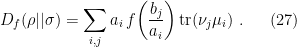
 are only independently orthonormal (that is, it does not follow that
  ). Accordingly, consider performing sequential measurement
  with
with  . This can be used to constructed the
  , where
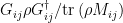 with probability
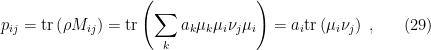
 . Let us denote the probabilities associated with the outcomes of acting on
  . Solving for the eigenvalues
  and
and  in these expressions then enables one rewrite
  ,
,  , whereupon we find
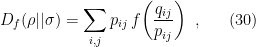
 for any smooth convex function
 , where
  . In fact, for a simple measurement which diagonalizes
  coincides precisely with the Fisher metric and
  -connections. Additionally, note that
  ; in other words, for arbitrary vector fields
 is formally understood as the vector field such that
  . Thus
  ,
,  are indeed invariant under the action of
  . Then for
  , we obtain
![\displaystyle D^{(\alpha)}(\rho||\sigma)=\frac{4}{1-\alpha^2}\left[1-\mathrm{tr}\left(\rho^{\frac{1-\alpha}{2}}\sigma^{\frac{1+\alpha}{2}}\right)\right]~, \ \ \ \ \ (33)](https://s0.wp.com/latex.php?latex=%5Cdisplaystyle+D%5E%7B%28%5Calpha%29%7D%28%5Crho%7C%7C%5Csigma%29%3D%5Cfrac%7B4%7D%7B1-%5Calpha%5E2%7D%5Cleft%5B1-%5Cmathrm%7Btr%7D%5Cleft%28%5Crho%5E%7B%5Cfrac%7B1-%5Calpha%7D%7B2%7D%7D%5Csigma%5E%7B%5Cfrac%7B1%2B%5Calpha%7D%7B2%7D%7D%5Cright%29%5Cright%5D%7E%2C+%5C+%5C+%5C+%5C+%5C+%2833%29&bg=ffffff&fg=000000&s=0&c=20201002)
![\displaystyle D^{(-1)}(\rho||\sigma)=D^{(1)}(\sigma||\rho)=\mathrm{tr}\left[\rho\left(\ln\rho-\ln\sigma\right)\right]~, \ \ \ \ \ (34)](https://s0.wp.com/latex.php?latex=%5Cdisplaystyle+D%5E%7B%28-1%29%7D%28%5Crho%7C%7C%5Csigma%29%3DD%5E%7B%281%29%7D%28%5Csigma%7C%7C%5Crho%29%3D%5Cmathrm%7Btr%7D%5Cleft%5B%5Crho%5Cleft%28%5Cln%5Crho-%5Cln%5Csigma%5Cright%29%5Cright%5D%7E%2C+%5C+%5C+%5C+%5C+%5C+%2834%29&bg=ffffff&fg=000000&s=0&c=20201002)


 -power and logarithm of an operator
  are defined such that these become
  and
and  , respectively, with the same (original) orthonormal eigenvectors. Of course, the quantum analogue of the Kullback-Leibler divergence
  , and the canonical divergence is the (quantum) relative entropy
  . And as in the
  -autoparallel submanifold
  as
as![\displaystyle \rho_\theta=\mathrm{exp}\left[C+\theta^iF_i-\psi(\theta)\right]~, \ \ \ \ \ (37)](https://s0.wp.com/latex.php?latex=%5Cdisplaystyle+%5Crho_%5Ctheta%3D%5Cmathrm%7Bexp%7D%5Cleft%5BC%2B%5Ctheta%5EiF_i-%5Cpsi%28%5Ctheta%29%5Cright%5D%7E%2C+%5C+%5C+%5C+%5C+%5C+%2837%29&bg=ffffff&fg=000000&s=0&c=20201002)
 are hermitian operators, and
  -valued function on the canonical parameters
 ![{[\theta^i]}](https://s0.wp.com/latex.php?latex=%7B%5B%5Ctheta%5Ei%5D%7D&bg=ffffff&fg=000000&s=0&c=20201002) . As in the classical case, these form a 1-affine coordinate system, and hence the dual
. As in the classical case, these form a 1-affine coordinate system, and hence the dual  , which naturally extends the classical definition in terms of the expectation value of
  , cf. eq. (36) of
 ![{[\eta_i]}](https://s0.wp.com/latex.php?latex=%7B%5B%5Ceta_i%5D%7D&bg=ffffff&fg=000000&s=0&c=20201002) are related through the dual potential
are related through the dual potential  , defined via the Legendre transform
![\displaystyle \varphi(\theta)=\mathrm{sup}_{\theta'}\left[\theta'^i\eta_i(\theta)-\psi(\theta')\right]~. \ \ \ \ \ (38)](https://s0.wp.com/latex.php?latex=%5Cdisplaystyle+%5Cvarphi%28%5Ctheta%29%3D%5Cmathrm%7Bsup%7D_%7B%5Ctheta%27%7D%5Cleft%5B%5Ctheta%27%5Ei%5Ceta_i%28%5Ctheta%29-%5Cpsi%28%5Ctheta%27%29%5Cright%5D%7E.+%5C+%5C+%5C+%5C+%5C+%2838%29&bg=ffffff&fg=000000&s=0&c=20201002)
 , where the derivative is with respect to
  . But this condition precisely corresponds to the definition of
  above, cf. eq. (37) in
 , and used the fact that
  ).
).
 (i.e., a quantum channel), and operator convex function
  , and provides a definition of relative entropy even for type-III factors. For finite-dimensional systems, one can show that this reduces precisely to the familiar definition of quantum relative entropy given above. For more details, I warmly recommend the recent review by Witten [2]. Additionally, the fact that
  reads
reads
 parametrizes the transverse directions. Now consider the action for a bulk scalar
 . The on-shell equations of motion yield the familiar Klein-Gordon equation,
 scale like
  , where
  are given by
 . The general solution to the Klein-Gordon equation in the limit
  may therefore be expressed as a linear combination of these solutions, with coefficients
  and
and  :
: ![\displaystyle \phi(z,\mathbf{x})\rightarrow z^{\Delta_+}\left[A(\mathbf{x})+O(z^2)\right]+z^{\Delta_-}\left[B(\mathbf{x})+O(z^2)\right]~. \ \ \ \ \ (5)](https://s0.wp.com/latex.php?latex=%5Cdisplaystyle+%5Cphi%28z%2C%5Cmathbf%7Bx%7D%29%5Crightarrow+z%5E%7B%5CDelta_%2B%7D%5Cleft%5BA%28%5Cmathbf%7Bx%7D%29%2BO%28z%5E2%29%5Cright%5D%2Bz%5E%7B%5CDelta_-%7D%5Cleft%5BB%28%5Cmathbf%7Bx%7D%29%2BO%28z%5E2%29%5Cright%5D%7E.+%5C+%5C+%5C+%5C+%5C+%285%29&bg=ffffff&fg=000000&s=0&c=20201002)
 behaviour plays no role in the following, so we’ll suppress it henceforth.
 imposes a limit on the allowed mass of the bulk field, namely that
  . This is known as the Breitenlohner-Freedman (BF) bound. (Unlike in flat space, a negative mass squared doesn’t necessarily imply that the theory is unstable; intuitively, the negative curvature of AdS compensates for the backreaction, provided the excitations are sufficiently small). Furthermore, if one integrates the action
  to the cutoff at
  , the result will be finite for
  , i.e.,
  . Thus
  is a solution for all masses above the BF bound.
 , the situation is slightly more subtle. One can show that the boundary term obtained by integrating
  ; i.e., for
  , which corresponds to the restricted mass range
 corresponds to the constraint, from unitarity, on the representation of conformal field theories. Hence for masses below the unitarity bound (but above the BF bound, of course), one may choose either
  by definition, the second term dominates in the
  in order that the solution be normalizable—though as remarked above, this is clearly not the full story in the mass range
  , whereupon one sees that
 . But it does not explain why
 is the bulk-boundary propagator with conformal dimension
 ![\displaystyle K_\Delta(z,\mathbf{x},\mathbf{x}')=\pi^{-d/2}\frac{\Gamma(\Delta)}{\Gamma(\Delta-d/2)}\frac{z^\Delta}{\left[z^2+(\mathbf{x}-\mathbf{x}')^2\right]^\Delta}~, \ \ \ \ \ (10)](https://s0.wp.com/latex.php?latex=%5Cdisplaystyle+K_%5CDelta%28z%2C%5Cmathbf%7Bx%7D%2C%5Cmathbf%7Bx%7D%27%29%3D%5Cpi%5E%7B-d%2F2%7D%5Cfrac%7B%5CGamma%28%5CDelta%29%7D%7B%5CGamma%28%5CDelta-d%2F2%29%7D%5Cfrac%7Bz%5E%5CDelta%7D%7B%5Cleft%5Bz%5E2%2B%28%5Cmathbf%7Bx%7D-%5Cmathbf%7Bx%7D%27%29%5E2%5Cright%5D%5E%5CDelta%7D%7E%2C+%5C+%5C+%5C+%5C+%5C+%2810%29&bg=ffffff&fg=000000&s=0&c=20201002)
 is the boundary limit of the bulk field
  , and
, and
 , whence
![\displaystyle Z[J]=\exp\left(\frac{i}{2}\int\!\mathrm{d}^dx\mathrm{d}^dx'J(\mathbf{x})G(\mathbf{x},\mathbf{x}')J(\mathbf{x}')\right)~, \ \ \ \ \ (13)](https://s0.wp.com/latex.php?latex=%5Cdisplaystyle+Z%5BJ%5D%3D%5Cexp%5Cleft%28%5Cfrac%7Bi%7D%7B2%7D%5Cint%5C%21%5Cmathrm%7Bd%7D%5Edx%5Cmathrm%7Bd%7D%5Edx%27J%28%5Cmathbf%7Bx%7D%29G%28%5Cmathbf%7Bx%7D%2C%5Cmathbf%7Bx%7D%27%29J%28%5Cmathbf%7Bx%7D%27%29%5Cright%29%7E%2C+%5C+%5C+%5C+%5C+%5C+%2813%29&bg=ffffff&fg=000000&s=0&c=20201002)
![\displaystyle \langle\mathcal{O}(\mathbf{x}_1)\ldots\mathcal{O}(\mathbf{x}_n)\rangle=\frac{1}{i^n}\frac{\delta^nZ[J]}{\delta J(\mathbf{x}_1)\ldots\delta J(\mathbf{x}_n)}\bigg|_{J=0}~. \ \ \ \ \ (14)](https://s0.wp.com/latex.php?latex=%5Cdisplaystyle+%5Clangle%5Cmathcal%7BO%7D%28%5Cmathbf%7Bx%7D_1%29%5Cldots%5Cmathcal%7BO%7D%28%5Cmathbf%7Bx%7D_n%29%5Crangle%3D%5Cfrac%7B1%7D%7Bi%5En%7D%5Cfrac%7B%5Cdelta%5EnZ%5BJ%5D%7D%7B%5Cdelta+J%28%5Cmathbf%7Bx%7D_1%29%5Cldots%5Cdelta+J%28%5Cmathbf%7Bx%7D_n%29%7D%5Cbigg%7C_%7BJ%3D0%7D%7E.+%5C+%5C+%5C+%5C+%5C+%2814%29&bg=ffffff&fg=000000&s=0&c=20201002)
![\displaystyle \frac{1}{i}\frac{\delta Z[J]}{\delta J(\mathbf{x})}\bigg|_{J=0}=\int\!\mathrm{d}^dx'J(\mathbf{x})G(\mathbf{x},\mathbf{x}')Z[J]\bigg|_{J=0}=\langle\mathcal{O}(\mathbf{x})\rangle~, \ \ \ \ \ (15)](https://s0.wp.com/latex.php?latex=%5Cdisplaystyle+%5Cfrac%7B1%7D%7Bi%7D%5Cfrac%7B%5Cdelta+Z%5BJ%5D%7D%7B%5Cdelta+J%28%5Cmathbf%7Bx%7D%29%7D%5Cbigg%7C_%7BJ%3D0%7D%3D%5Cint%5C%21%5Cmathrm%7Bd%7D%5Edx%27J%28%5Cmathbf%7Bx%7D%29G%28%5Cmathbf%7Bx%7D%2C%5Cmathbf%7Bx%7D%27%29Z%5BJ%5D%5Cbigg%7C_%7BJ%3D0%7D%3D%5Clangle%5Cmathcal%7BO%7D%28%5Cmathbf%7Bx%7D%29%5Crangle%7E%2C+%5C+%5C+%5C+%5C+%5C+%2815%29&bg=ffffff&fg=000000&s=0&c=20201002)
 and
and  , thus explaining the relation
  ). Of course, setting
  causes the one-point function to vanish on-shell. The fact that we set the sources to zero resolves the apparent tension between setting
  on-shell.
 simply interchanges these roles. It is an interesting and under-appreciated fact that any holographic CFT therefore admits two different bulk duals, i.e., two different quantum field theories are encoded in the same CFT Lagrangian!

 is irrelevant (
![{[h]<0}](https://s0.wp.com/latex.php?latex=%7B%5Bh%5D%3C0%7D&bg=ffffff&fg=000000&s=0&c=20201002) ), then the deformation does not change the effective field theory, since it only plays a role in high-energy correlators. However, if the coupling is relevant (
), then the deformation does not change the effective field theory, since it only plays a role in high-energy correlators. However, if the coupling is relevant (![{[h]>0}](https://s0.wp.com/latex.php?latex=%7B%5Bh%5D%3E0%7D&bg=ffffff&fg=000000&s=0&c=20201002) ), then the perturbation induces a flow into the IR. And it turns out that the boundary conditions change from
), then the perturbation induces a flow into the IR. And it turns out that the boundary conditions change from  , where
  . Thus in the UV, we choose
  to be dimensionless, we must have
 ![{[h]=d-2\Delta}](https://s0.wp.com/latex.php?latex=%7B%5Bh%5D%3Dd-2%5CDelta%7D&bg=ffffff&fg=000000&s=0&c=20201002) . The condition that
. The condition that  . Since

 and
and  , which amounts to a trivial relabeling of the variables in this expression. However, the alternative quantization, in which
  and
and  , is slightly more subtle: a similar relabeling would work for the present case, but not for a multi-trace deformation. Instead, consider varying the effective action with respect to the operator
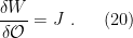
 , then invariance of the generating functional
 ![{Z[J]}](https://s0.wp.com/latex.php?latex=%7BZ%5BJ%5D%7D&bg=ffffff&fg=000000&s=0&c=20201002) requires
requires![\displaystyle 0=\delta Z[J]=i\int\!\mathcal{D}\phi\,e^{iS}\int\!\mathrm{d}^dx\left(\frac{\delta S}{\delta \phi(x)}+J(x)\right)\delta\phi(x)~, \ \ \ \ \ (21)](https://s0.wp.com/latex.php?latex=%5Cdisplaystyle+0%3D%5Cdelta+Z%5BJ%5D%3Di%5Cint%5C%21%5Cmathcal%7BD%7D%5Cphi%5C%2Ce%5E%7BiS%7D%5Cint%5C%21%5Cmathrm%7Bd%7D%5Edx%5Cleft%28%5Cfrac%7B%5Cdelta+S%7D%7B%5Cdelta+%5Cphi%28x%29%7D%2BJ%28x%29%5Cright%29%5Cdelta%5Cphi%28x%29%7E%2C+%5C+%5C+%5C+%5C+%5C+%2821%29&bg=ffffff&fg=000000&s=0&c=20201002)

 — in particular, that it should be identified with
 for consistency with the cited literature (and the convenient factor of 2). According to
 as the energy scale
  . Since
  ,
,  , with the standard choice
  , and hence we identify
  -algebra
  of observables in some spacetime region
  is a von Neumann algebra. Recall that a
  by von Neumann’s double commutant theorem. Additionally, we take
  ,
,  are dense in
  iff
iff  . (Note that, glossing over various
  of
of  . The commutant is then the algebra in the left Rindler wedge
  ,
,  . (The very last equality is sometimes called Haag duality, and applies when
  are causal complements).
 , which we will use to derive some relationships between the left and right Rindler wedges. The starting point is the antilinear map
  , defined by
 between complex vector spaces
  satisfies
  and
and  . Note that
  is a state-dependent operator, in that it is defined in terms of its action on the cyclic and separating state
  such that
  but
but  , which contradicts the definition (1). The fact that
  that, as an operator, we must have
  . Note that by the square of the operator, we do not mean
  ; rather, this implies that
  . It turns out that
  , the corresponding operator on the commutant
  .
.
 ) called the modular conjugation, and
  , implies that
 such that
 such that
  . Our notation here is consistent with [2,3]). Since both
  leave the vacuum state invariant, this property extends to the modular operator as well,
  . It it important to note that
  is
is  , but this does not contradict the fact that
 in conjunction with the polar decomposition. Combining (5) with the aforementioned fact that
  leads to
  and
and  . Finally, expressing

 ,
,  such that
 ![{[\mathcal{O},\mathcal{O}']=0}](https://s0.wp.com/latex.php?latex=%7B%5B%5Cmathcal%7BO%7D%2C%5Cmathcal%7BO%7D%27%5D%3D0%7D&bg=ffffff&fg=000000&s=0&c=20201002) . The isomorphism (8) is rather remarkable: it allows one to map operators between the left and right Rindler wedges, and features crucially in the works of Papadodimas and Raju on reconstructing black hole interiors [2,3].
. The isomorphism (8) is rather remarkable: it allows one to map operators between the left and right Rindler wedges, and features crucially in the works of Papadodimas and Raju on reconstructing black hole interiors [2,3]. be a unitary operator with support in
  ) in
) in 


 is an operator in the commutant. Indistinguishably of
  from the vacuum for observers in
  ! This is due to the fact, mentioned above, that
  . This example highlights the subtle yet crucial distinction between localized states vs. localized operators. Another way to emphasize this is that, as operators,

 , but in the course of doing so it provides some insight into where and why this factorization fails, and highlights which operators do and do not exist—the reduced density matrix for either wedge being a prime example of the latter.
 half-plane which produces the vacuum state
  . Stitching these together by integrating over all boundary values at
  . As we shall shortly see, this is related to the modular operator
 at
at  ,
,  . Strictly speaking, this defines
  , but taking the weak closure to construct the associated von Neumann algebras entails including the bifurcation point
 indicates that we identify the fields in the upper and lower half-plane when computing the partial trace, while the cut along
  are kept free. The regularization issue mentioned above arises from the fact that local operators at the boundary point
  are not well-defined, but must be treated as smeared distributions over some finite region. In typical calculations of entanglement entropy, one excises some small region around the endpoint of the cut, which acts as a UV cutoff that regulates the divergent result. [I am grateful to Jamie Sully for discussions on this issue]. But we can’t strictly do this while preserving the (von Neumann) algebraic structure above, which is one reason this procedure doesn’t rigorously hold.
 in the Euclidean
  plane:
 plane with boost parameter
  , and we know that the generator of such a boost can be expressed as
 . Now if the factorization of the Hilbert space were legitimate, we could split
  (with domains of integration restricted to the associated wedges), such that the path integral over the wedge in figure (c) yields the operator
  , where
  . Such an operator propagates degrees of freedom from the upper boundary of the wedge at
  to the lower boundary. By setting
  , one sees that we recover the path integral in figure (b), and therefore
 generating
  . We then recover the modular operator
 ![{[M_L,M_R]=0}](https://s0.wp.com/latex.php?latex=%7B%5BM_L%2CM_R%5D%3D0%7D&bg=ffffff&fg=000000&s=0&c=20201002) , and hence
, and hence
 (note that many authors absorb the factor of
  maps states in
  removes a wedge of angle
  thus moves an operator insertion from
  cannot be split into
  in such a way as to yield operators whose support lies solely in
  . This implies that the reduced density matrices
  do not really exist! Given how much of our understanding of entanglement in quantum field theory is based on the reduced density matrix — and more recently, at least in certain holographic applications, the modular Hamiltonian
  itself — this is in principle a rather serious problem. It remains to be seen how much of our ideas about entanglement must accordingly be revised, or whether this is analagous to Haag’s theorem about the non-existence of the interaction picture: theoretically damning, but practically irrelevant.
 . The non-existence of the operator
  manifests in a universal UV divergence in
  at
at  are still well-defined. An intuitive argument for this is that in the energy eigenbasis, correlation functions between well-defined (read: finite) states simply don’t see the problematic UV modes. [I am grateful to Ben Freivogel for this explanation]. Of course, one could certainly inquire as to the ontological status of matrix elements of an operator which does not technically exist. But, at least at an epistemic level, this offers a potential back-door to entanglement entropy. That is, taking the trace of the reduced density matrix
  and
and  . In particular, the cases
  are intimately related to two important families of statistical models, the exponential or e-family with affine connection
  , and the mixed or m-family with affine connection
  . Hence before turning to general aspects of the dual structure on
  be a finite set. As before, an arbitrary model

 , which implies that
  is specifically an open subset of the affine subspace
 is naturally identified with the linear subspace
 , considered as elements of
  , will be denoted
 then defines the
 ![{\xi=[\xi^i]}](https://s0.wp.com/latex.php?latex=%7B%5Cxi%3D%5B%5Cxi%5Ei%5D%7D&bg=ffffff&fg=000000&s=0&c=20201002) , with
, with  , with respect to which
  , i.e.,
 makes the affine structure, and in particular the significance of the
  , and identify
  . Elements
  and call this the exponential or e-representation. In local coordinates, we have
  . By the chain rule,
 is obtained by modifying the constraint on
 ![{0=\sum\nolimits_xp(x)A(x)=E_p[A]}](https://s0.wp.com/latex.php?latex=%7B0%3D%5Csum%5Cnolimits_xp%28x%29A%28x%29%3DE_p%5BA%5D%7D&bg=ffffff&fg=000000&s=0&c=20201002) , i.e.,
, i.e.,![\displaystyle T_p^{(e)}\mathcal{P}\equiv\left\{X^{(e)}\,\Big|\,X\in T_p\mathcal{P}\right\} =\{A\in\mathcal{R}^\mathcal{X}\,|\,E_p[A]=0\}~. \ \ \ \ \ (8)](https://s0.wp.com/latex.php?latex=%5Cdisplaystyle+T_p%5E%7B%28e%29%7D%5Cmathcal%7BP%7D%5Cequiv%5Cleft%5C%7BX%5E%7B%28e%29%7D%5C%2C%5CBig%7C%5C%2CX%5Cin+T_p%5Cmathcal%7BP%7D%5Cright%5C%7D+%3D%5C%7BA%5Cin%5Cmathcal%7BR%7D%5E%5Cmathcal%7BX%7D%5C%2C%7C%5C%2CE_p%5BA%5D%3D0%5C%7D%7E.+%5C+%5C+%5C+%5C+%5C+%288%29&bg=ffffff&fg=000000&s=0&c=20201002)
 ,
,  does not generally belong to
  for
for  , the constraint in (7) implies that the shifted vector
 ![{A'\equiv A-E_q[A]}](https://s0.wp.com/latex.php?latex=%7BA%27%5Cequiv+A-E_q%5BA%5D%7D&bg=ffffff&fg=000000&s=0&c=20201002) does belong to
does belong to ![\displaystyle \Pi_{p,q}^{(e)}X=X'\;\;\mathrm{such~that}\;\;{X'}^{(e)}=X^{(e)}-E_q[X^{(e)}]~, \ \ \ \ \ (9)](https://s0.wp.com/latex.php?latex=%5Cdisplaystyle+%5CPi_%7Bp%2Cq%7D%5E%7B%28e%29%7DX%3DX%27%5C%3B%5C%3B%5Cmathrm%7Bsuch%7Ethat%7D%5C%3B%5C%3B%7BX%27%7D%5E%7B%28e%29%7D%3DX%5E%7B%28e%29%7D-E_q%5BX%5E%7B%28e%29%7D%5D%7E%2C+%5C+%5C+%5C+%5C+%5C+%289%29&bg=ffffff&fg=000000&s=0&c=20201002)
 denotes parallel transport with respect to the e-connection
  . (Properly showing that
  leads naturally to the e-affine coordinate system and associated connection introduced in the previous
 ![\displaystyle \langle X,Y\rangle_p=E_p\left[X^{(e)}Y^{(e)}\right]~. \ \ \ \ \ (10)](https://s0.wp.com/latex.php?latex=%5Cdisplaystyle+%5Clangle+X%2CY%5Crangle_p%3DE_p%5Cleft%5BX%5E%7B%28e%29%7DY%5E%7B%28e%29%7D%5Cright%5D%7E.+%5C+%5C+%5C+%5C+%5C+%2810%29&bg=ffffff&fg=000000&s=0&c=20201002)
![{E_p[A]}](https://s0.wp.com/latex.php?latex=%7BE_p%5BA%5D%7D&bg=ffffff&fg=000000&s=0&c=20201002) to perturbations of
to perturbations of ![\displaystyle V_p[A]=E_p[(A-E_p[A])^2]=||(\mathrm{d} E[A])_p||_p^2~, \ \ \ \ \ (11)](https://s0.wp.com/latex.php?latex=%5Cdisplaystyle+V_p%5BA%5D%3DE_p%5B%28A-E_p%5BA%5D%29%5E2%5D%3D%7C%7C%28%5Cmathrm%7Bd%7D+E%5BA%5D%29_p%7C%7C_p%5E2%7E%2C+%5C+%5C+%5C+%5C+%5C+%2811%29&bg=ffffff&fg=000000&s=0&c=20201002)
 is the differential of
  is “loose enough” for this to be possible, but this constraint becomes increasingly strict as the cardinality of
  , but in fact this extends to general
  , which Amari & Nagaoka call a dualistic structure on

 , and similarly for
  etc. Given a metric
  . Additionally, the combination
  is metric. Conversely, one immediately sees that the condition for
  , and in this sense dual connections simply constitute a more general class thereof.
 from
from  with respect to
  and
and  . As mentioned in the previous
 such that
  , with equality iff
  . While this provides a measure of the separation between
![{[g_{ij}^{(D)}]}](https://s0.wp.com/latex.php?latex=%7B%5Bg_%7Bij%7D%5E%7B%28D%29%7D%5D%7D&bg=ffffff&fg=000000&s=0&c=20201002) is a positive definite matrix everywhere on
is a positive definite matrix everywhere on  via
via
 . We can also define an affine connection
  associated with this divergence, via the coefficients

 , from which we have
  and
and  . Thus we have that
  are dual with respect to
  . In fact, any dual structure
 with
with  . The f-divergence satisfies a number of important properties (see page 56), chief of which is monotonicity under arbitrary probability transition functions. That is, let
  be randomly transformed into
  with probability
  , with
  . This maps distributions
  to
to  , respectively. Monotonicity of the f-divergence is then the statement that
 is a generalization of the deterministic mapping induced by
  in the previous
  . Consequently, the equality is saturated iff
  .
. , defined for all
  via
via

 -flatness of
  a dually flat space. Such spaces have a number of properties that are closely related to various concepts in statistics.
![{[\eta_j]}](https://s0.wp.com/latex.php?latex=%7B%5B%5Ceta_j%5D%7D&bg=ffffff&fg=000000&s=0&c=20201002) , respectively, in which vector fields are denoted
, respectively, in which vector fields are denoted  and
and  . Since both
  are flat, the condition on parallel transport (14) implies that
  is in fact constant on
 ![{[\eta^j]}](https://s0.wp.com/latex.php?latex=%7B%5B%5Ceta%5Ej%5D%7D&bg=ffffff&fg=000000&s=0&c=20201002) such that
such that
 , then the connections

 that satisfies the following partial differential equation:
 , and hence the second derivatives of
 . These two functions are related via
 , whereupon substituting in (27) one recovers (28). Now, the form of (29) — equivalently, the pair (27) and (28) — suggests that
 ![\displaystyle \varphi(q)=\mathrm{sup}_{p\in S}\left[\theta^i(p)\eta_i(q)-\psi(p)\right]\quad\mathrm{and}\quad \psi(p)=\mathrm{sup}_{q\in S}\left[\theta^i(p)\eta_i(q)-\varphi(q)\right]~. \ \ \ \ \ (30)](https://s0.wp.com/latex.php?latex=%5Cdisplaystyle+%5Cvarphi%28q%29%3D%5Cmathrm%7Bsup%7D_%7Bp%5Cin+S%7D%5Cleft%5B%5Ctheta%5Ei%28p%29%5Ceta_i%28q%29-%5Cpsi%28p%29%5Cright%5D%5Cquad%5Cmathrm%7Band%7D%5Cquad+%5Cpsi%28p%29%3D%5Cmathrm%7Bsup%7D_%7Bq%5Cin+S%7D%5Cleft%5B%5Ctheta%5Ei%28p%29%5Ceta_i%28q%29-%5Cvarphi%28q%29%5Cright%5D%7E.+%5C+%5C+%5C+%5C+%5C+%2830%29&bg=ffffff&fg=000000&s=0&c=20201002)


 , with equality iff
 and
and  with
with  due to the
  .
.![\displaystyle p(x;\theta)=\exp\left[C(x)+\theta^iF_i(x)-\psi(\theta)\right]~, \ \ \ \ \ (35)](https://s0.wp.com/latex.php?latex=%5Cdisplaystyle+p%28x%3B%5Ctheta%29%3D%5Cexp%5Cleft%5BC%28x%29%2B%5Ctheta%5EiF_i%28x%29-%5Cpsi%28%5Ctheta%29%5Cright%5D%7E%2C+%5C+%5C+%5C+%5C+%5C+%2835%29&bg=ffffff&fg=000000&s=0&c=20201002)
![\displaystyle \eta_i=\eta_i(\theta)\equiv E_\theta[F_i]=\int\!\mathrm{d} x\,F_i(x)p(x;\theta)~. \ \ \ \ \ (36)](https://s0.wp.com/latex.php?latex=%5Cdisplaystyle+%5Ceta_i%3D%5Ceta_i%28%5Ctheta%29%5Cequiv+E_%5Ctheta%5BF_i%5D%3D%5Cint%5C%21%5Cmathrm%7Bd%7D+x%5C%2CF_i%28x%29p%28x%3B%5Ctheta%29%7E.+%5C+%5C+%5C+%5C+%5C+%2836%29&bg=ffffff&fg=000000&s=0&c=20201002)
![\displaystyle 0=E_\theta[\partial_i\ell_\theta]=E_\theta[F_i(x)-\partial_i\psi(\theta)]\;\;\implies\;\; \eta_i=\partial_i\psi~. \ \ \ \ \ (37)](https://s0.wp.com/latex.php?latex=%5Cdisplaystyle+0%3DE_%5Ctheta%5B%5Cpartial_i%5Cell_%5Ctheta%5D%3DE_%5Ctheta%5BF_i%28x%29-%5Cpartial_i%5Cpsi%28%5Ctheta%29%5D%5C%3B%5C%3B%5Cimplies%5C%3B%5C%3B+%5Ceta_i%3D%5Cpartial_i%5Cpsi%7E.+%5C+%5C+%5C+%5C+%5C+%2837%29&bg=ffffff&fg=000000&s=0&c=20201002)
![{g_{ij}(\theta)=-E_\theta[\partial_i\partial_j\ell_\theta]}](https://s0.wp.com/latex.php?latex=%7Bg_%7Bij%7D%28%5Ctheta%29%3D-E_%5Ctheta%5B%5Cpartial_i%5Cpartial_j%5Cell_%5Ctheta%5D%7D&bg=ffffff&fg=000000&s=0&c=20201002) implies that for an exponential family,
implies that for an exponential family,  and
and  for the example of the normal distribution in the previous
  is identified with the parameters:
![\displaystyle \begin{aligned} \mathcal{X}=&\{x_0,\ldots,x_n\}~,\qquad \Xi=\left\{[\xi^i]\,\Big|\,\xi^i>0\;\;\forall i~,\;\;\sum_{i=1}^n\xi^i<1\right\}\\ &p(x_i;\xi)=\begin{cases} \xi^i & 1\leq i\leq n \\ 1-\sum_{i=1}^n\xi^i\quad & i=0 \end{cases}~. \end{aligned} \ \ \ \ \ (38)](https://s0.wp.com/latex.php?latex=%5Cdisplaystyle+%5Cbegin%7Baligned%7D+%5Cmathcal%7BX%7D%3D%26%5C%7Bx_0%2C%5Cldots%2Cx_n%5C%7D%7E%2C%5Cqquad+%5CXi%3D%5Cleft%5C%7B%5B%5Cxi%5Ei%5D%5C%2C%5CBig%7C%5C%2C%5Cxi%5Ei%3E0%5C%3B%5C%3B%5Cforall+i%7E%2C%5C%3B%5C%3B%5Csum_%7Bi%3D1%7D%5En%5Cxi%5Ei%3C1%5Cright%5C%7D%5C%5C+%26p%28x_i%3B%5Cxi%29%3D%5Cbegin%7Bcases%7D+%5Cxi%5Ei+%26+1%5Cleq+i%5Cleq+n+%5C%5C+1-%5Csum_%7Bi%3D1%7D%5En%5Cxi%5Ei%5Cquad+%26+i%3D0+%5Cend%7Bcases%7D%7E.+%5Cend%7Baligned%7D+%5C+%5C+%5C+%5C+%5C+%2838%29&bg=ffffff&fg=000000&s=0&c=20201002)

![\displaystyle \varphi(\theta)=E_\theta[\ln p_\theta-C]=-H(p_\theta)-E_\theta[C]~, \ \ \ \ \ (41)](https://s0.wp.com/latex.php?latex=%5Cdisplaystyle+%5Cvarphi%28%5Ctheta%29%3DE_%5Ctheta%5B%5Cln+p_%5Ctheta-C%5D%3D-H%28p_%5Ctheta%29-E_%5Ctheta%5BC%5D%7E%2C+%5C+%5C+%5C+%5C+%5C+%2841%29&bg=ffffff&fg=000000&s=0&c=20201002)
 is the entropy!
 . We wish to consider the problem of estimating the unknown parameter
  by some function
  of the data
 ![{[\hat\xi^i]:\mathcal{X}\rightarrow\mathbb{R}^n}](https://s0.wp.com/latex.php?latex=%7B%5B%5Chat%5Cxi%5Ei%5D%3A%5Cmathcal%7BX%7D%5Crightarrow%5Cmathbb%7BR%7D%5En%7D&bg=ffffff&fg=000000&s=0&c=20201002) is called an estimator. Furthermore,
is called an estimator. Furthermore,  is an unbiased estimator if
![\displaystyle E_\xi[\hat\xi(X)]=\xi\quad\forall\xi\in\Xi~, \ \ \ \ \ (42)](https://s0.wp.com/latex.php?latex=%5Cdisplaystyle+E_%5Cxi%5B%5Chat%5Cxi%28X%29%5D%3D%5Cxi%5Cquad%5Cforall%5Cxi%5Cin%5CXi%7E%2C+%5C+%5C+%5C+%5C+%5C+%2842%29&bg=ffffff&fg=000000&s=0&c=20201002)
![{V_\xi[\hat\xi]=[v_\xi^{ij}]}](https://s0.wp.com/latex.php?latex=%7BV_%5Cxi%5B%5Chat%5Cxi%5D%3D%5Bv_%5Cxi%5E%7Bij%7D%5D%7D&bg=ffffff&fg=000000&s=0&c=20201002) , whose elements are defined via
, whose elements are defined via![\displaystyle v_\xi^{ij}\equiv E_\xi\left[(\hat\xi^i(X)-\xi^i)(\hat\xi^j(X)-\xi^j)\right]~. \ \ \ \ \ (43)](https://s0.wp.com/latex.php?latex=%5Cdisplaystyle+v_%5Cxi%5E%7Bij%7D%5Cequiv+E_%5Cxi%5Cleft%5B%28%5Chat%5Cxi%5Ei%28X%29-%5Cxi%5Ei%29%28%5Chat%5Cxi%5Ej%28X%29-%5Cxi%5Ej%29%5Cright%5D%7E.+%5C+%5C+%5C+%5C+%5C+%2843%29&bg=ffffff&fg=000000&s=0&c=20201002)
![\displaystyle V_\xi[\hat\xi]\geq G(\xi)^{-1}~, \ \ \ \ \ (44)](https://s0.wp.com/latex.php?latex=%5Cdisplaystyle+V_%5Cxi%5B%5Chat%5Cxi%5D%5Cgeq+G%28%5Cxi%29%5E%7B-1%7D%7E%2C+%5C+%5C+%5C+%5C+%5C+%2844%29&bg=ffffff&fg=000000&s=0&c=20201002)
![{V_\xi[\hat\xi]-G(\xi)^{-1}}](https://s0.wp.com/latex.php?latex=%7BV_%5Cxi%5B%5Chat%5Cxi%5D-G%28%5Cxi%29%5E%7B-1%7D%7D&bg=ffffff&fg=000000&s=0&c=20201002) is a positive semidefinite matrix. An unbiased estimator
is a positive semidefinite matrix. An unbiased estimator  to have an efficient estimator is that
  to make contact with the notation just introduced. Then the condition (0.36) implies that
  is in fact an unbiased estimator for
  and
and ![\displaystyle g_{ij}(\theta)=E_\theta[(F_i-\eta_i)(F_j-\eta_j)]~, \ \ \ \ \ (45)](https://s0.wp.com/latex.php?latex=%5Cdisplaystyle+g_%7Bij%7D%28%5Ctheta%29%3DE_%5Ctheta%5B%28F_i-%5Ceta_i%29%28F_j-%5Ceta_j%29%5D%7E%2C+%5C+%5C+%5C+%5C+%5C+%2845%29&bg=ffffff&fg=000000&s=0&c=20201002)
![{V_\eta[\hat\eta]=G=[g_{ij}]}](https://s0.wp.com/latex.php?latex=%7BV_%5Ceta%5B%5Chat%5Ceta%5D%3DG%3D%5Bg_%7Bij%7D%5D%7D&bg=ffffff&fg=000000&s=0&c=20201002) , and hence
, and hence 