As part of one of my current research projects, I’ve been looking into variational autoencoders (VAEs) for the purpose of identifying and analyzing attractor solutions within higher-dimensional phase spaces. Of course, I couldn’t resist diving into the deeper mathematical theory underlying these generative models, beyond what was strictly necessary in order to implement one. As in the case of the restricted Boltzmann machines I’ve discussed before, there are fascinating relationships between physics, information theory, and machine learning at play here, in particular the intimate connection between (free) energy minimization and Bayesian inference. Insofar as I actually needed to learn how to build one of these networks however, I’ll start by introducing VAEs from a somewhat more implementation-oriented mindset, and discuss the deeper physics/information-theoretic aspects afterwards.

Mathematical formulation

An autoencoder is a type of neural network (NN) consisting of two feedforward networks: an encoder, which maps an input onto a latent space , and a decoder, which maps the latent representation to the output . The idea is that , so that information in the original data is compressed into a lower-dimensional “feature space”. For this reason, autoencoders are often used for dimensional reduction, though their applicability to real-world problems seems rather limited. Training consists of minimizing the difference between and according to some suitable loss function. They are a form of unsupervised (or rather, self-supervised) learning, in which the NN seeks to learn highly compressed, discrete representation of the input.

VAEs inherit the network structure of autoencoders, but are fundamentally rather different in that they learn the parameters of a probability distribution that represents the data. This makes them much more powerful than their simpler precursors insofar as they are generative models (that is, they can generate new examples of the input type). Additionally, their statistical nature — in particular, learning a continuous probability distribution — makes them vastly superior in yielding meaningful results from new/test data that gets mapped to novel regions of the latent space. In a nutshell, the encoding is generated stochastically, using variational techniques—and we’ll have more to say on what precisely this means below.

Mathematically, a VAE is a latent-variable model with latent variables and observed variables (i.e., data) , where represents the parameters of the distribution. (For example, Gaussian distributions are uniquely characterized by their mean and standard deviation , in which case ; more generally, would parametrize the masses and couplings of whatever model we wish to construct. Note that we shall typically suppress the subscript where doing so does not lead to ambiguity). This joint distribution can be written

The first factor on the right-hand side is the decoder, i.e., the likelihood of observing given ; this provides the map from . This will typically be either a multivariate Gaussian or Bernoulli distribution, implemented by an RBM with as-yet unlearned weights and biases. The second factor is the prior distribution of latent variables , which will be related to observations via the likelihood function (i.e., the decoder). This can be thought of as a statement about the variable with the data held fixed. In order to be computational tractable, we want to make the simplest possible choice for this distribution; accordingly, one typically chooses a multivariate Gaussian,

In the context of Bayesian inference, this is technically what’s known as an informative prior, since it assumes that any other parameters in the model are sufficiently small that Gaussian sampling from does not miss any strongly relevant features. This is in contrast to the somewhat misleadingly named uninformative prior, which endeavors to place no subjective constraints on the variable; for this reason, the latter class are sometimes called objective priors, insofar as they represent the minimally biased choice. In any case, the reason such a simple choice (2) suffices for is that any distribution can be generated by applying a sufficiently complicated function to the normal distribution.

Meanwhile, the encoder is represented by the posterior probability , i.e., the probability of given ; this provides the map from . In principle, this is given by Bayes’ rule:

but this is virtually impossible to compute analytically, since the denominator amounts to evaluating the partition function over all possible configurations of latent variables, i.e.,

One solution is to compute approximately via Monte Carlo sampling; but the impression I’ve gained from my admittedly superficial foray into the literature is that such models are computationally expensive, noisy, difficult to train, and generally inferior to the more elegant solution offered by VAEs. The key idea is that for most , , so instead of sampling over all possible , we construct a new distribution representing the values of which are most likely to have produced , and sample over this new, smaller set of values [2]. In other words, we seek a more tractable approximation , characterized by some other, variational parameters —so-called because we will eventually vary these parameters in order to ensure that is as close to as possible. As usual, the discrepancy between these distributions is quantified by the familiar Kullback-Leibler (KL) divergence:

where the subscript on the left-hand side denotes the variable over which we marginalize.

This divergence plays a central role in the variational inference procedure we’re trying to implement, and underlies the connection to the information-theoretic relations alluded above. Observe that Bayes’ rule enables us to rewrite this expression as

where denotes the expectation value with respect to , and we have used the fact that (since probabilities are normalized to 1, and has no dependence on the latent variables ). Now observe that the first term on the right-hand side can be written as another KL divergence. Rearranging, we therefore have

where we have identified the (negative) variational free energy

As the name suggests, this is closely related to the Helmholtz free energy from thermodynamics and statistical field theory; we’ll discuss this connection in more detail below, and in doing so provide a more intuitive definition: the form (8) is well-suited to the implementation-oriented interpretation we’re about to provide, but is a few manipulations removed from the underlying physical meaning.

The expressions (7) and (8) comprise the central equation of VAEs (and variational Bayesian methods more generally), and admit a particularly simple interpretation. First, observe that the left-hand side of (7) is the log-likelihood, minus an “error term” due to our use of an approximate distribution . Thus, it’s the left-hand side of (7) that we want our learning procedure to maximize. Here, the intuition underlying maximum likelihood estimation (MLE) is that we seek to maximize the probability of each under the generative process provided by the decoder . As we will see, the optimization process pulls towards via the KL term; ideally, this vanishes, whereupon we’re directly optimizing the log-likelihood .

The variational free energy (8) consists of two terms: a reconstruction error given by the expectation value of with respect to , and a so-called regulator given by the KL divergence. The reconstruction error arises from encoding into using our approximate distribution , whereupon the log-likelihood of the original data given these inferred latent variables will be slightly off. The KL divergence, meanwhile, simply encourages the approximate posterior distribution to be close to , so that the encoding matches the latent distribution. Note that since the KL divergence is positive-definite, (7) implies that the negative variational free energy gives a lower-bound on the log-likelihood. For this reason, is sometimes referred to as the Evidence Lower BOund (ELBO) by machine learners.

The appearance of the (variational) free energy (8) is not a mere mathematical coincidence, but stems from deeper physical aspects of inference learning in general. I’ll digress upon this below, as promised, but we’ve a bit more work to do first in order to be able to actually implement a VAE in code.

Computing the gradient of the cost function

Operationally, training a VAE consists of performing stochastic gradient descent (SGD) on (8) in order to minimize the variational free energy (equivalently, maximize the ELBO). In other words, this will provide the cost or loss function (9) for the model. Note that since is constant with respect to , (7) implies that minimizing the variational energy indeed forces the approximate posterior towards the true posterior, as mentioned above.

In applying SGD to the cost function (8), we actually have two sets of parameters over which to optimize: the parameters that define the VAE as a generative model , and the variational parameters that define the approximate posterior . Accordingly, we shall write the cost function as

where, to avoid a preponderance of subscripts, we shall continue to denote , and similarly . Taking the gradient with respect to is easy, since only the first term on the right-hand side has any dependence thereon. Hence, for a given datapoint ,

where in the second step we have replaced the expectation value with a single sample drawn from the latent space . This is a common method in SGD, in which we take this particular value of to be a reasonable approximation for the average . (Yet-more connections to mean field theory (MFT) we must of temporal necessity forgo; see Mehta et al. [1] for some discussion in this context, or Doersch [2] for further intuition). The resulting gradient can then be computed via backpropagation through the NN.

The gradient with respect to , on the other hand, is slightly problematic, since the variational parameters also appear in the distribution with respect to which we compute expectation values. And the sampling trick we just employed means that in the implementation of this layer of the NN, the evaluation of the expectation value is a discrete operation: it has no gradient, and hence we can’t backpropagate through it. Fortunately, there’s a clever method called the reparametrization trick that circumvents this stumbling block. The basic idea is to change variables so that no longer appears in the distribution with respect to which we compute expectation values. To do so, we express the latent variable (which is ostensibly drawn from ) as a differentiable and invertible transformation of some other, independent random variable , i.e., (where here “independent” means that the distribution of does not depend on either or ; typically, one simply takes ). We can then replace , whereupon we can move the gradient inside the expectation value as before, i.e.,

Note that in principle, this results in an additional term due to the Jacobian of the transformation. Explicitly, this equivalence between expectation values may be written

where the Jacobian has been absorbed into the definition of :

Consequently, the Jacobian would contribute to the second term of the KL divergence via

Operationally however, the reparametrization trick simply amounts to performing the requisite sampling on an additional input layer for instead of on ; this is nicely illustrated in both fig. 74 of Mehta et al. [1] and fig. 4 of Doersch [2]. In practice, this means that the analytical tractability of the Jacobian is a non-issue, since the change of variables is performed downstream of the KL divergence layer—see the implementation details below. The upshot is that while the above may seem complicated, it makes the calculation of the gradient tractable via standard backpropagation.

Implementation

Having fleshed-out the mathematical framework underlying VAEs, how do we actually build one? Let’s summarize the necessary ingredients, layer-by-layer along the flow from observation space to latent space and back (that is, ), with the Keras API in mind:

• We need an input layer, representing the data .
• We connect this input layer to an encoder, , that maps data into the latent space . This will be a NN with an arbitrary number of layers, which outputs the parameters of the distribution (e.g., the mean and standard deviation, if is Gaussian).
• We need a special KL-divergence layer, to compute the second term in the cost function (8) and add this to the model’s loss function (e.g., the Keras loss). This takes as inputs the parameters produced by the encoder, and our Gaussian ansatz (2) for the prior .
• We need another input layer for the independent distribution . This will be merged with the parameters output by the encoder, and in this way automatically integrated into the model’s loss function.
• Finally, we feed this merged layer into a decoder, , that maps the latent space back to . This is generally another NN with as many layers as the encoder, which relies on the learned parameters of the generative model.

At this stage of the aforementioned research project, it’s far too early to tell whether such a VAE will ultimately be useful for accomplishing our goal. If so, I’ll update this post with suitable links to paper(s), etc. But regardless, the variational inference procedure underling VAEs is interesting in its own right, and I’d like to close by discussing some of the physical connections to which I alluded above in greater detail.

Deeper connections

The following was largely inspired by the exposition in Mehta et al. [1], though we have endeavored to modify the notation for clarity/consistency. In particular, be warned that what these authors call the “free energy” is actually a dimensionless free energy, which introduces an extra factor of (cf. eq. (158) therein); we shall instead stick to standard conventions, in which the mass dimension is . Of course, we’re eventually going to set anyway, but it’s good to set things straight.

Consider a system of interacting degrees of freedom , with parameters (e.g., for Gaussians, or would parametrize the couplings between spins in the Ising model). We may assign an energy to each configuration, such that the probability of finding the system in a given state at temperature is

where the partition function with respect to this ensemble is

where the sum runs over both and . As the notation suggests, we have in mind that will serve as our latent-variable model, in which respectively take on the meanings of visible and latent degrees of freedom as above. Upon marginalizing over the latter, we recover the partition function (4) for finite:

where in the last step, we have defined the marginalized energy function that encodes all interactions with the latent variables; cf. eq. (15) of our post on RBMs.

The above implies that the posterior probability of finding a particular value of , given the observed value (i.e., the encoder) can be written as

where

is the hamiltonian that describes the interactions between and , in which the -independent contributions have been subtracted off; cf. the difference between eq. (12) and (15) here. To elucidate the variational inference procedure however, it will be convenient to re-express the conditional distribution as

where we have defined and such that

where the subscript will henceforth be used to refer to the posterior distribution, as opposed to either the joint or prior (this to facilitate a more compact notation below). Here, is precisely the partition function we encountered in (4), and is independent of the latent variable . Statistically, this simply reflects the fact that in (20), we weight the joint probabilities by how likely the condition is to occur. Meanwhile, one must be careful not to confuse with above. Rather, comparing (21) with (15), we see that represents a sort of renormalized energy, in which the partition function has been absorbed.

Now, in thermodynamics, the Helmholtz free energy is defined as the difference between the energy and the entropy (with a factor of for dimensionality) at constant temperature and volume, i.e., the work obtainable from the system. More fundamentally, it is the (negative) log of the partition function of the canonical ensemble. Hence for the encoder (18), we write

where is the expectation value with respect to and marginalization over (think of these as internal degrees of freedom), and is the corresponding entropy,

Note that given the canonical form (18), the equivalence of these expressions for — that is, the second equality in (22) — follows immediately from the definition of entropy:

where, since has no explicit dependence on the latent variables, . As usual, this partition function is generally impossible to calculate. To circumvent this, we employ the strategy introduced above, namely we approximate the true distribution by a so-called variational distribution , where are the variational (e.g., coupling) parameters that define our ansatz. The idea is of course that should be computationally tractable while still capturing the essential features. As alluded above, this is the reason these autoencoders are called “variational”: we’re eventually going to vary the parameters in order to make as close to as possible.

To quantify this procedure, we define the variational free energy (not to be confused with the Helmholtz free energy (22)):

where is the expectation value of the energy corresponding to the distribution with respect to . While the variational energy has the same form as the thermodynamic definition of Helmholtz energy , it still seems odd at first glance, since it no longer enjoys the statistical connection to a canonical partition function. To gain some intuition for this quantity, suppose we express our variational distribution in the canonical form, i.e.,

where we have denoted the energy of configurations in this ensemble by , to avoid confusion with , cf. (18). Then may be written

Thus we see that the variational energy is indeed formally akin to the Helmholtz energy, except that it encodes the difference in energy between the true and approximate configurations. We can rephrase this in information-theoretic language by expressing these energies in terms of their associated ensembles; that is, we write 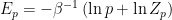, and similarly for , whereupon we have

where the terms have canceled. Recognizing (5) and (21) on the right-hand side, we therefore find that the difference between the variational and Helmholtz free energies is none other than the KL divergence,

which is precisely (7)! (It is perhaps worth stressing that this follows directly from (24), independently of whether takes canonical form).

As stated above, our goal in training the VAE is to make the variational distribution as close to as possible, i.e., minimizing the KL divergence between them. We now see that physically, this corresponds to a variational problem in which we seek to minimize with respect to . In the limit where we perfectly succeed in doing so, has obtained its global minimum , whereupon the two distributions are identical.

Finally, it remains to clarify our implementation-based definition of given in (8) (where ). Applying Bayes’ rule, we have

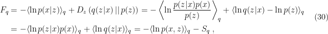
which is another definition of sometimes found in the literature, e.g., as eq. (172) of Mehta et al. [1]. By expressing in terms of via (20), we see that this is precisely equivalent to our more thermodynamical definition (24). Alternatively, we could have regrouped the posteriors to yield

where the identification of follows from (20). Of course, this is just (28) again, which is a nice check on internal consistency.

References

1. The review by Mehta et al., A high-bias, low-variance introduction to Machine Learning for physicists is absolutely perfect for those with a physics background, and the accompanying Jupyter notebook on VAEs in Keras for the MNIST dataset was especially helpful for the implementation bits above. The latter is a more streamlined version of this blog post by Louis Tiao.
2. Doersch has written a Tutorial on Autoencoders, which I found helpful for gaining some further intuition for the mapping between theory and practice.