The issue of boundary conditions in AdS/CFT has confused me for years; not because it’s intrinsically complicated, but because most of the literature simply regurgitates a superficial explanation for the standard prescription which collapses at the first inquiry. Typically, the story is presented as follows. Since we’ll be interested in the near-boundary behaviour of bulk fields, it is convenient to work in the Poincaré patch, in which the metric for Euclidean AdS reads

where parametrizes the transverse directions. Now consider the action for a bulk scalar , dual to some primary operator in the CFT:

where . The on-shell equations of motion yield the familiar Klein-Gordon equation,

This is a second-order differential equation with two independent solutions, whose leading behaviour as one approaches the boundary at scale like , where are given by

For compactness, we shall henceforth set the AdS radius . The general solution to the Klein-Gordon equation in the limit may therefore be expressed as a linear combination of these solutions, with coefficients and :

The subleading behaviour plays no role in the following, so we’ll suppress it henceforth.

Note that the condition imposes a limit on the allowed mass of the bulk field, namely that . This is known as the Breitenlohner-Freedman (BF) bound. (Unlike in flat space, a negative mass squared doesn’t necessarily imply that the theory is unstable; intuitively, the negative curvature of AdS compensates for the backreaction, provided the excitations are sufficiently small). Furthermore, if one integrates the action (2) from to the cutoff at , the result will be finite for , i.e., . Thus is a solution for all masses above the BF bound.

For , the situation is slightly more subtle. One can show that the boundary term obtained by integrating (2) by parts is non-zero only if ; i.e., for , there exists a second, inequivalent action (read: theory). And in this case, the bulk integral up to the cutoff is finite only for , which corresponds to the restricted mass range

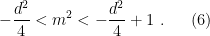
The upper limit is called the unitarity bound, since the limit corresponds to the constraint, from unitarity, on the representation of conformal field theories. Hence for masses below the unitarity bound (but above the BF bound, of course), one may choose either or , which implies two different bulk theories for the same CFT. More on this below. (Slightly more technical details can be found in section 5.3 of [1]).

With the above in hand, the vast majority of the literature simply recites the “standard prescription”, in which one identifies as the source of the boundary operator , which is in turn identified with . This appears to be based on the observation that, since by definition, the second term dominates in the limit, which requires that one set in order that the solution be normalizable—though as remarked above, this is clearly not the full story in the mass range (6). Sometimes, an attempt is made to justify this identification by the observation that one can multiply through by , whereupon one sees that

In accordance with the extrapolate dictionary, this indeed suggests that sources the bulk field . But it does not explain why should be identified as the boundary dual of this bulk field; that is, it does not explain why and should be related in the CFT action as

since a priori these are independent coefficients appearing in the solution to the differential equation above. Furthermore, it does not follow from the fact that the bulk coefficient has the correct conformal dimension as the boundary source field (and that both will be set to zero on-shell) that the two must be identified: this may be aesthetically suggestive, but it is by no means logically necessary.

Some clarification is found in the classic paper by Klebanov and Witten [2]. They observe that the extrapolate dictionary — or what one would identify, in more modern language, as the HKLL prescription for bulk reconstruction — can be written

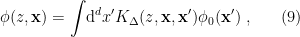
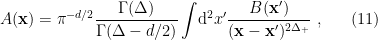
where is the bulk-boundary propagator with conformal dimension ,

and is the boundary limit of the bulk field , which serves as the source for the dual operator . Choosing then implies that in order to be consistent with (5), we must identify , and

which one obtains by taking the limit of the integral above. We then recognize the position-space Green function , whence

which is the statement that is the source for the one-point function . That is, recall that the generating function can be written in terms of the Feynman propagator as

whereupon the functional derivative with respect to the source yields the -point function

Hence, taking a single derivative, we have

which is precisely the form of (12), with and , thus explaining the relation (8). (Note that we’re ignoring a constant factor here; the exact relation between and the vev is fixed in [2] to ). Of course, setting causes the one-point function to vanish on-shell. The fact that we set the sources to zero resolves the apparent tension between setting for normalizability, and simultaneously having it appear in (12): the expansion (5) was obtained by solving the equations of motion, so we only have on-shell.

Thus we see that the bulk-boundary correspondence in the form (9) provides the extra constraint needed to relate the coefficients and in the expansion (5) as (vev of) operator and source, respectively, and that choosing the alternative boundary condition simply interchanges these roles. It is an interesting and under-appreciated fact that any holographic CFT therefore admits two different bulk duals, i.e., two different quantum field theories are encoded in the same CFT Lagrangian!

The above essentially summarizes the basic story for the usual case, i.e., a CFT action of the form

However, the question I encountered during my research that actually motivated this post is what happens to these boundary conditions in the presence of a double-trace deformation,

To that end, suppose we start with a CFT at some UV fixed point. If the coupling is irrelevant (), then the deformation does not change the effective field theory, since it only plays a role in high-energy correlators. However, if the coupling is relevant (), then the perturbation induces a flow into the IR. And it turns out that the boundary conditions change from (in the UV) to (in the IR) as a result.

First, let’s understand why we need to start with the “alternative boundary condition” in the UV. The paper [3] motivates this by examining the Green function in momentum space, which scales like , where . Thus in the UV, we choose so that the Green function converges. This explanation isn’t entirely satisfactory though, since it’s not clear why this should converge with in the IR.

In this sense, a better explanation for choosing in the UV is obtained simply by examining the mass dimensions in the coupling term (17): in order for to be dimensionless, we must have . The condition that be a relevant coupling then implies that . Since can only satisfy this condition for masses below the Breitenlohner-Freedman bound, we are constrained to choose . Note that from this perspective, the choice is equally valid, but it corresponds to an irrelevant perturbation instead, so nothing interesting happens.

Understanding why the theory flows to at the new IR fixed point is more complicated, and requires computing the beta functions for the couplings. This is done in [4], where they compute the evolution equation for the coupling (i.e., the beta function for ), which enables them to identify the fixed points which correspond to the alternative and standard quantizations in the UV and IR, respectively.

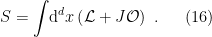
It is then natural to ask what happens at intermediate points along the flow, since the above applies only to the UV/IR fixed points, at which a single choice (either or ) is determined. This leads to the notion of mixed boundary conditions, as introduced by Witten in [5]. In order to understand his proposal, let’s examine the relationship between and above from another angle. The term in the effective action corresponding to the single-trace insertion is

Taking functional derivatives with respect to the source then yields the operator expectation value,

which of course simply restates the relationship (15). As explained above, the standard quantization identifies and , which amounts to a trivial relabeling of the variables in this expression. However, the alternative quantization, in which and , is slightly more subtle: a similar relabeling would work for the present case, but not for a multi-trace deformation. Instead, consider varying the effective action with respect to the operator :

Note that unlike (19), this is an operator statement; it may seem like an odd thing to write down, but in fact it’s formally the same expression that arises in the derivation of Ward identities. Specifically, if one considers an infinitesimal shift of the field variable , then invariance of the generating functional requires

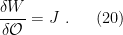
where we’ve taken the action (16) with in place of . The resemblance to Noether’s theorem is intriguing, but I’m not sure whether there’s a deeper relation to symmetries in QFT at work here. In any case, Witten’s proposal is that in the alternative quantization, one should identify

which simply states that . Strictly speaking, we can’t identify in this expression, since it doesn’t tell us the vev of the operator . Rather, to find the expectation value — in particular, that it should be identified with — requires us to solve the bulk equations of motion with this boundary condition, substitute the result into the bulk action, and then take variational derivatives with respect to the source as usual. In the end of course, one recovers the simple identification , hence Witten actually writes (22) directly with in place of , with the understanding that the expression is purely formal.

Now consider a double-trace deformation,

where we’ve rescaled the coupling for consistency with the cited literature (and the convenient factor of 2). According to (22), this leads to the mixed boundary condition

As observed in [3], this neatly interpolates between the standard and alternative prescriptions above. To see this, observe that since the deformation is explicitly chosen to be relevant, the dimensionless coupling grows as we move into the IR, i.e., 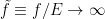as the energy scale . Since , (5) requires that we identify , with the standard choice . Conversely, the coupling shrinks to zero in the UV, where , and hence we identify as the vev of the operator instead, with the alternative choice .

Witten’s prescription extends to higher-trace deformations as well, though I won’t discuss those here. The point, for the purposes of the present post, is that it provides a unified treatment of boundary conditions in holography that smoothly interpolates between the UV/IR, and hence allows one to naturally treat the bulk dual all along the flow.

I am grateful to my former officemate, Diptarka Das, for several enlightening discussions on this topic, and for graciously allowing me to pester him across several afternoons until I was satisfied.

References

- M. Ammon and J. Erdmenger, “Gauge/gravity duality,” Cambridge University Press, Cambridge, 2015.
- I. R. Klebanov and E. Witten, “AdS / CFT correspondence and symmetry breaking,” Nucl. Phys. B556 (1999) 89–114, arXiv:hep-th/9905104 [hep-th].
- T. Hartman and L. Rastelli, “Double-trace deformations, mixed boundary conditions and functional determinants in AdS/CFT,” JHEP 01 (2008) 019, arXiv:hep-th/0602106 [hep-th].
- I. Heemskerk and J. Polchinski, “Holographic and Wilsonian Renormalization Groups,” JHEP 06 (2011) 031, arXiv:1010.1264 [hep-th].
- E. Witten, “Multitrace operators, boundary conditions, and AdS / CFT correspondence,” arXiv:hep-th/0112258 [hep-th].