Information geometry (part 3/3)

Insofar as quantum mechanics can be regarded as an extension of (classical) probability theory, most of the concepts developed in the previous two parts of this sequence can be extended to quantum information theory as well, thus giving rise to quantum information geometry.

Quantum preliminaries

Let’s first review a few basic quantum mechanical notions; we’ve covered this in more detail before, but it will be helpful to establish present notation/language.

Quantum mechanics is the study of linear operators acting on some complex Hilbert space ${\mathcal{H}}$ . We shall take this to be finite-dimensional, and hence identify ${\mathcal{H}=\mathbb{C}^k}$ , the space of ${k\!\times\!k}$ complex matrices, where ${k=\mathrm{dim}\,\mathcal{H}}$ . In the usual bra-ket notation, the adjoint ${A^*}$ of an operator ${A}$ is defined by ${\langle x|Ay\rangle=\langle A^*x|y\rangle}$ for all vectors ${x,y}$ . The density operator ${\rho}$ , which describes a quantum state, is a postive semidefinite hermitian operator of unit trace. ${\rho}$ is a pure state if it is of rank 1 (meaning it admits a representation of the form ${\rho=|x\rangle\langle x|}$ ), and mixed otherwise.

A measurement ${\Pi=\{\pi_i\}=\{\pi_1,\ldots,\pi_n\}}$ is a set of operators on ${\mathcal{H}}$ which satisfy

$\displaystyle \pi_i=\pi_i^*\geq0\qquad\mathrm{and}\qquad\sum_i\pi_i=1~, \ \ \ \ \ (1)$

whose action on the state ${\rho}$ yields the outcome ${e_i\in\{e_1,\ldots,e_n\}}$ with probability

$\displaystyle P(e_i)=\mathrm{tr}{\rho\pi_i}~. \ \ \ \ \ (2)$

Note that by virtue of (1), ${P\{e_i\}}$ is a probability distribution:

$\displaystyle P(e_i)\geq0\qquad\mathrm{and}\qquad\sum_iP(e_i)=1~. \ \ \ \ \ (3)$

If we further impose that ${\Pi}$ consist of orthogonal projections, i.e.,

$\displaystyle \pi_i\pi_j=\pi_i\delta_{ij}~, \ \ \ \ \ (4)$

then the above describes a “simple measurement”, or PVM (projection-valued measure). More generally of course, a measurement is described by a POVM (positive operator-valued measure). We covered this concept in an earlier post, but the distinction will not be relevant here.

An observable is formally defined as the pair ${(\{\pi_i\},\{a_i\})}$ , where ${a_i\in\mathbb{R}}$ is a real number associated with the measurement outcome ${e_i}$ . Since ${\{\pi_i\}}$ are orthogonal projectors, we may represent the observable as a (hermitian) operator ${A}$ acting on ${\mathcal{H}}$ whose associated eigenvalues are ${\{a_i\}}$ , i.e.,

$\displaystyle A=\sum_ia_i\pi_i~. \ \ \ \ \ (5)$

The expectation and variance of ${A}$ in the state ${\rho}$ are then

$\displaystyle E_\rho[A]=\sum_i\mathrm{tr}{\rho\pi_i}a_i=\mathrm{tr}{\rho A}~, \ \ \ \ \ (6)$

$\displaystyle V_\rho[A]=\sum_i\mathrm{tr}{\rho\pi_i}\left(a_i-E_\rho[A]\right)^2=\mathrm{tr}\!\left[\rho\left(A-E_\rho[A]\right)^2\right]~. \ \ \ \ \ (7)$

We shall denote the set of all operators ${A}$ on ${\mathcal{H}}$ by

$\displaystyle \mathcal{A}=\{A\,|\,A=A^*\}~, \ \ \ \ \ (8)$

and define

$\displaystyle \mathcal{A}_1\equiv\{A\in\mathcal{A}\,|\,\mathrm{tr}A=1\}\subset\mathcal{A}~. \ \ \ \ \ (9)$

Then the set of all density operators ${\rho}$ is a convex subset of ${\mathcal{A}_1}$ :

$\displaystyle \bar{\mathcal{S}}\equiv\{\rho\,|\,\rho=\rho^*\geq0\;\;\mathrm{and}\;\;\mathrm{tr}\rho=1\}~. \ \ \ \ \ (10)$

Note the similarities with the embedding formalism introduced in the previous post. The set of density operators admits a partition based on the rank of the matrix,

$\displaystyle \bar{\mathcal{S}}=\bigcup_{r=1}^k\mathcal{S}_r~,\qquad\mathrm{where}\qquad \mathcal{S}_r\equiv\{\rho\in\bar{\mathcal{S}}\,|\,\mathrm{rank}\,\rho=r\}~. \ \ \ \ \ (11)$

Pure states are then elements of ${\mathcal{S}_1}$ , which form the extreme points of the convex set ${\bar{\mathcal{S}}}$ (i.e., they cannot be represented as convex combinations of other points, which is the statement that ${\rho=|x\rangle\langle x|}$ ). Geometrically, the pure states are the vertices of the convex hull, while the (strictly positive) mixed states ${\rho\in\mathcal{S}_{r>1}}$ lie in the interior.

We need one more preliminary notion, namely the set ${\mathcal{U}}$ of unitary operators on ${\mathcal{H}}$ :

$\displaystyle \mathcal{U}=\{U\,|\,U^{-1}=U^*\}~. \ \ \ \ \ (12)$

This forms a Lie group, whose action on ${\bar{\mathcal{S}}}$ is given by

$\displaystyle \mathcal{U}\times\bar{\mathcal{S}}\rightarrow\bar{\mathcal{S}}\qquad\mathrm{where}\qquad (U,\rho)\mapsto U\rho U^{-1}\equiv\tilde\rho~. \ \ \ \ \ (13)$

(The first expression says that the group multiplication by ${U}$ sends elements of ${\bar{\mathcal{S}}}$ to ${\bar{\mathcal{S}}}$ , while the second specifies how this mapping acts on individual elements). Since the matrix rank is preserved, each ${\mathcal{S}_r}$ is closed under the action of ${\mathcal{U}}$ . It follows from (13) that ${\mathcal{U}}$ maps measurements ${\Pi}$ and observables ${A}$ to

$\displaystyle \tilde\pi_i=U\pi_i U^{-1}\qquad\mathrm{and}\qquad\tilde A=UAU^{-1}~, \ \ \ \ \ (14)$

and that the probability distributions and expectation values are therefore invariant, i.e.,

$\displaystyle \mathrm{tr}(\tilde\rho\tilde\pi_i)=\mathrm{tr}(\rho\pi_i)\qquad\mathrm{and}\qquad \mathrm{tr}(\tilde\rho\tilde A)=\mathrm{tr}(\rho A)~. \ \ \ \ \ (15)$

Of course, this last is the familiar statement that the unitarity of quantum mechanics ensures that probabilities are preserved.

Geometric preliminaries

Now, on to (quantum information) geometry! Let us restrict our attention to ${\mathcal{S}_1}$ for now; we shall consider mixed states below. Recall that pure states are actually rays, not vectors, in Hilbert space. Since ${\mathcal{H}=\mathbb{C}^k}$ , we therefore identify ${\mathcal{S}_1=\mathbb{C}P^{k-1}}$ (i.e., the pure states are in one-to-one correspondence with the rays in ${\mathbb{C}^{k}}$ , where we’ve projected out by the physically irrelevant phase). We now wish to associate a metric to this space of states; in particular, we seek a Riemannian metric which is invariant under unitary transformations ${\mathcal{U}}$ . It turns out that, up to an overall constant, this is uniquely provided by the Fubini-Study metric. Recall that when considering classical distributions, we found that the Fisher metric was the unique Riemannian metric that preserved the inner product. The Fubini-Study metric is thus the natural extension of the Fisher metric to the quantum mechanical case (for pure states only!). Unfortunately, Amari & Nagaoka neither define nor discuss this entity, but it’s reasonably well-known in the quantum information community, and has recently played a role in efforts to define holographic complexity in field theories. A particularly useful expression in this context is

$\displaystyle \mathrm{d}s^2=\langle\psi|\partial_\sigma U^\dagger\partial_\sigma U|\psi\rangle -\big|\langle\psi|U^\dagger\partial_\sigma U|\psi\rangle\big|^2~, \ \ \ \ \ (16)$

where ${\sigma\in\mathbb{R}}$ parametrizes the unitary ${U(\sigma)}$ that performs the transformation between states in ${\mathcal{S}_1}$ .

In the remainder of this post, we shall follow Amari & Nagaoka (chapter 7) in considering only mixed states; accordingly, for convenience, we hence forth denote ${\mathcal{S}_{r>1}}$ by simply ${\mathcal{S}}$ , i.e.,

$\displaystyle \mathcal{S}\equiv\{\rho\,|\,\rho=\rho^*>0\;\;\mathrm{and}\;\;\mathrm{tr}\rho=1\}~. \ \ \ \ \ (17)$

This is an open subset of ${\mathcal{A}_1}$ , and thus we may regard it as a real manifold of dimension ${n\equiv\mathrm{dim}\mathcal{A}_1}$ . Since the dimension of ${\mathcal{H}}$ is given by the number of linearly independent basis vectors, minus 1 for the trace constraint, ${n=k^2\!-\!1}$ . The tangent space ${T_\rho\mathcal{S}}$ at a point ${\rho}$ is then identified with

$\displaystyle \mathcal{A}_0\equiv\{A\in\mathcal{A}\,|\,\mathrm{tr}A=0\}~. \ \ \ \ \ (18)$

Note that this precisely parallels the embedding formalism used in defining the m-representation. Hence we denote a tangent vector ${X\in T_\rho\mathcal{S}}$ by ${X^{(m)}}$ , and call it the m-representation of ${X}$ in analogy with the classical case. (We’ll come to the quantum analogue of the e-representation later).

The PVM ${\Pi}$ introduced above can also be represented in geometrical terms, via the submanifold

$\displaystyle \mathcal{S}_\Pi=\mathcal{S}\,\cap\,\left\{\sum_{i=1}^la_i\pi_i\,\Big|\,(a_1,\ldots,a_l)\in\mathbb{R}^l\right\} =\left\{\sum_{i=1}^l\frac{p_i}{\mathrm{tr}\,\pi_i}\pi_i\,\Big|\,p=(p_1,\ldots,p_l)\in\mathcal{P}_l\right\}~. \ \ \ \ \ (19)$

That is, ${\mathcal{S}_\Pi}$ is the intersection of two sets. The first, ${\mathcal{S}\subset\mathcal{A}_1}$ , is simply the set of all operators ${A}$ with unit trace. From (5), we recognize the second as the spectral representation of operators in the eigenbasis of ${\Pi}$ . Imposing the trace constraint then implies that the eigenvalues of ${A}$ are weighted probabilities, where 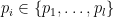${p_i\in\{p_1,\ldots,p_l\}}$ and ${\mathcal{P}_l=\mathcal{P}\{1,\ldots,l\}}$ is the totality of positive probability distributions ${p\equiv P\{e_i\}}$ with ${i\in[1,l]}$ . To see this, observe that

$\displaystyle \mathrm{tr}\sum_ia_i\pi_i =\sum_i\mathrm{tr}(\pi_i)a_i=1\;\implies\; a_i=\frac{p_i}{\mathrm{tr}(\pi_i)}~, \ \ \ \ \ (20)$

since ${\sum p_i=1}$ ; this underlies the second equality in the expression for ${\mathcal{S}_\Pi}$ above.

Lastly, the action of a unitary ${U\in\mathcal{U}}$ at a point ${\rho}$ results in a new vector, given by the mapping (13), which lives in (a subspace of) the tangent space ${T_\rho\mathcal{S}\simeq\mathcal{A}_0}$ . Such elements may be written

$\displaystyle \frac{\mathrm{d}}{\mathrm{d}t}U_t\rho U_t^{-1}\Big|_{t=0}=[\Omega,\rho]~, \ \ \ \ \ (21)$

where ${U_t\in\mathcal{U}}$ is a curve in the space of unitaries with ${U_0=1}$ , and ${\Omega}$ is its derivative at ${t=0}$ (note that ${t}$ corresponds to ${\sigma}$ in the expression for the Fubini-Study metric (16) above).

With the above notions in hand, we may now proceed to introduce a dual structure ${(g,\nabla,\nabla^*)}$ on ${\mathcal{S}}$ , and thereby the quantum analogues of the ${\alpha}$ -connections, divergence, etc.

Quantum divergences

In part 2 of this sequence, we introduced the f-divergence, which satisfies a number of desireable properties such as monotonicity. It also serves as the super-class to which the ${\alpha}$ -divergence belongs; the latter is particularly important, since it induces the dual structure consisting of the Fisher metric and ${(\pm\alpha)}$ -connections, and reduces to the familiar Kullback-Leibler divergence (a.k.a. relative entropy) for ${\alpha=\pm1}$ . We shall now introduce the quantum analogue of the f-divergence.

Denote by ${\mathcal{B}}$ the set of all (not necessarily hermitian) operators on ${\mathcal{H}}$ . Then given two strictly postive density operators ${\rho,\sigma\in\mathcal{S}}$ , the relative modular operator ${\Delta=\Delta_{\sigma,\rho}:\mathcal{B}\rightarrow\mathcal{B}}$ is defined by

$\displaystyle \Delta A=\sigma A\rho^{-1}~,\quad\forall A\in\mathcal{B}~. \ \ \ \ \ (22)$

Since ${\Delta}$ may be viewed as a hermitian and positive-definite operator on the Hilbert space, we may promote an arbitrary function ${f:\mathbb{R}^+\rightarrow\mathbb{R}}$ to a hermitian operator ${f(\Delta)}$ on said space such that

$\displaystyle \Delta A=\lambda A\;\implies\;f(\Delta)A=f(\lambda)A \quad\quad\forall\,\lambda\in\mathbb{R}^+,A\in\mathcal{B}~. \ \ \ \ \ (23)$

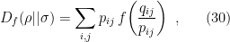
We then define the quantum f-divergence as

$\displaystyle D_f(\rho||\sigma)=\mathrm{tr}\left[\rho f(\Delta)\,1\right]~, \ \ \ \ \ (24)$

To see how this is consistent with (that is, reduces to) the classical f-divergence defined previously, consider the spectral representations

$\displaystyle \rho=\sum_ia_i\mu_i~,\quad\quad \sigma=\sum_ib_i\nu_i~, \ \ \ \ \ (25)$

where ${\{a_i\}}$ , ${\{b_i\}}$ are the eigenvalues for the PVMs ${\{\mu_i\}}$ , ${\{\nu_i\}}$ . Then from the definition of the relative modular operator above,

$\displaystyle \Delta(\nu_j\mu_j)=\frac{b_j}{a_i}\nu_j\mu_i \quad\implies\quad f(\nu_j\mu_j)=f\!\left(\frac{b_j}{a_i}\right)\nu_j\mu_i~, \ \ \ \ \ (26)$

and hence for simple measurements,

$\displaystyle D_f(\rho||\sigma)=\sum_{i,j}a_i\,f\!\left(\frac{b_j}{a_i}\right)\mathrm{tr}(\nu_j\mu_i)~. \ \ \ \ \ (27)$

To compare with the classical expression given in part 2 (cf. eq. (18)), we must take into account the fact that ${\mu}$ and ${\nu}$ are only independently orthonormal (that is, it does not follow that ${\mu_i\nu_j=\delta_{ij}\mu_i}$ ). Accordingly, consider performing sequential measurement ${\mu}$ followed by ${\nu}$ , i.e., ${G=\{G_{ij}\}}$ with ${G_{ij}=\nu_j\mu_i}$ . This can be used to constructed the POVM ${M=\{M_{ij}\}}$ , where

$\displaystyle M_{ij}=G_{ij}^\dagger G_{ij}=\mu_i\nu_j\mu_i~, \ \ \ \ \ (28)$

where we have used the orthonormality of ${\nu}$ . Applying von Neumann’s projection hypothesis, this takes the initial state ${\rho}$ to the final state 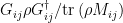${G_{ij}\rho G_{ij}^\dagger/\mathrm{tr}\left(\rho M_{ij}\right)}$ with probability

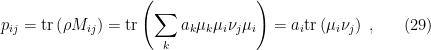
$\displaystyle p_{ij}=\mathrm{tr}\left(\rho M_{ij}\right) =\mathrm{tr}\left(\sum_ka_k\mu_k\mu_i\nu_j\mu_i\right) =a_i\mathrm{tr}\left(\mu_i\nu_j\right)~, \ \ \ \ \ (29)$

where in the last step we have again used the orthonormality condition (4), and the cyclic property of the trace. Similarly, by inverting this sequence of measurements, we may construct the POVM with elements ${N_{ij}=\nu_j\mu_i\nu_j}$ . Let us denote the probabilities associated with the outcomes of acting on ${\sigma}$ as ${q_{ij}=\mathrm{tr}\left(\sigma N_{ij}\right)=b_j\mathrm{tr}\left(\mu_i\nu_j\right)}$ . 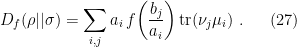Solving for the eigenvalues ${a_i}$ and ${b_j}$ in these expressions then enables one rewrite (27) in terms of the probability distributions ${p=\{p_{ij}\}}$ , ${q=\{q_{ij}\}}$ , whereupon we find

$\displaystyle D_f(\rho||\sigma)=\sum_{i,j}p_{ij}\,f\!\left(\frac{q_{ij}}{p_{ij}}\right)~, \ \ \ \ \ (30)$

which is the discrete analogue of the classical divergence referenced above.

Now, recall that every dual structure is naturally induced by a divergence. In particular, it follows from Chentsov’s theorem that the Fisher metric and ${\alpha}$ -connections are induced from the f-divergence ${D_f}$ for any smooth convex function ${f:\mathbb{R}^+\rightarrow\mathbb{R}}$ which satisfies

$\displaystyle f(1)=0~,\qquad f''(1)=1~,\qquad \alpha=3+2f'''(1)~. \ \ \ \ \ (31)$

Thus, to find the formal quantum analogues of these objects, we restrict to the class of functions ${f}$ which satisfy the above conditions, whereupon the quantum f-divergence ${D_f}$ induces the dual structure 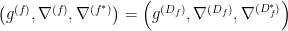${\left(g^{(f)},\nabla^{(f)},\nabla^{(f^*)}\right)=\left(g^{(D_f)},\nabla^{(D_f)},\nabla^{(D_f^*)}\right)}$ , where ${D_f^*=D_{f^*}}$ . In fact, for a simple measurement which diagonalizes ${\rho}$ , the restriction of this triple to ${S_\Pi}$ coincides precisely with the Fisher metric and ${\pm\alpha}$ -connections. Additionally, note that ${D_f}$ is invariant under unitary transformations, in the sense that ${D_f(U\rho U^*||U\sigma U^*)=D(\rho||\sigma)}$ ; in other words, for arbitrary vector fields ${X}$ , ${Y}$ , we have

$\displaystyle \langle UXU^*,UYU^*\rangle=\langle X,Y\rangle~, \ \ \ \ \ (32)$

where ${UXU^*}$ is formally understood as the vector field such that ${(UXU^*)_{U\rho U^*}^{(m)}=UX_\rho^{(m)}U^*}$ . Thus ${g=\langle\cdot,\cdot\rangle}$ , ${\nabla}$ , and ${\nabla^*}$ are indeed invariant under the action of ${U}$ , which is the characteristic property of the classical analogues we wanted to preserve.

As in the classical case, we can further restrict the class of functions ${f}$ to satisfy eq.~(20) in part 1, which defines the quantum ${\alpha}$ -divergence ${D^{(\alpha)}}$ . Then for ${\alpha\neq\pm1}$ , we obtain

$\displaystyle D^{(\alpha)}(\rho||\sigma)=\frac{4}{1-\alpha^2}\left[1-\mathrm{tr}\left(\rho^{\frac{1-\alpha}{2}}\sigma^{\frac{1+\alpha}{2}}\right)\right]~, \ \ \ \ \ (33)$

while for ${\alpha=\pm1}$ , we instead have

$\displaystyle D^{(-1)}(\rho||\sigma)=D^{(1)}(\sigma||\rho)=\mathrm{tr}\left[\rho\left(\ln\rho-\ln\sigma\right)\right]~, \ \ \ \ \ (34)$

cf. eq. (21) and (22) ibid. In obtaining these expressions, we used the fact that the relative modular operator satisfies

$\displaystyle (\Delta_{\sigma,\rho})^rA=\sigma^rA\rho^{-r}\quad\quad\forall r\in\mathbb{R} \ \ \ \ \ (35)$

and

$\displaystyle \left(\ln\Delta_{\sigma,\rho}\right)X=\left(\ln\sigma\right)X-X\ln\rho~, \ \ \ \ \ (36)$

where the ${r^{\mathrm{th}}}$ -power and logarithm of an operator ${\rho}$ with eigenvalues ${\{p_i\}}$ are defined such that these become ${\{p_i^r\}}$ and ${\{\ln p_i\}}$ , respectively, with the same (original) orthonormal eigenvectors. Of course, the quantum analogue of the Kullback-Leibler divergence (34) is none other than the quantum relative entropy!

Many of the classical geometric relations can also be extended to the quantum case. In particular, ${\mathcal{S}}$ is dually flat with respect to 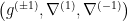${\left(g^{(\pm1)},\nabla^{(1)},\nabla^{(-1)}\right)}$ , and the canonical divergence is the (quantum) relative entropy ${D^{(\pm1)}}$ . And as in the discussion of (classical) exponential families, we can parameterize the elements of an arbitrary ${\nabla^{(1)}}$ -autoparallel submanifold ${M\subseteq\mathcal{S}}$ as

$\displaystyle \rho_\theta=\mathrm{exp}\left[C+\theta^iF_i-\psi(\theta)\right]~, \ \ \ \ \ (37)$

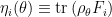where now ${F_1,\ldots,F_m}$ are hermitian operators, and ${\psi(\theta)}$ is an ${\mathbb{R}}$ -valued function on the canonical parameters ${[\theta^i]}$ . As in the classical case, these form a 1-affine coordinate system, and hence the dual ${(-1)}$ -affine coordinates are given by ${\eta_i(\theta)\equiv\mathrm{tr}\left(\rho_\theta F_i\right)}$ , which naturally extends the classical definition in terms of the expectation value of ${F_i}$ , cf. eq. (36) of part 2. Recall that ${[\theta^i]}$ and ${[\eta_i]}$ are related through the dual potential ${\varphi}$ , defined via the Legendre transform

$\displaystyle \varphi(\theta)=\mathrm{sup}_{\theta'}\left[\theta'^i\eta_i(\theta)-\psi(\theta')\right]~. \ \ \ \ \ (38)$

Taking a derivative of the bracketed quantity, the maximum occurs when ${\eta_i(\theta)=\partial_i\psi(\theta')}$ , where the derivative is with respect to ${\theta'^i}$ . But this condition precisely corresponds to the definition of ${\eta_i}$ above, cf. eq. (37) in part 2. Hence

$\displaystyle \varphi(\theta)=\theta^i\eta_i(\theta)-\psi(\theta) =-H(\rho_\theta)-\mathrm{tr}(\rho_\theta C)~, \ \ \ \ \ (39)$

where we have identified the von Neumann entropy ${H(\rho)\equiv-\mathrm{tr}(\rho\ln\rho)}$ , and used the fact that ${\mathrm{tr}\rho=1}$ (that is, ${\mathrm{tr}\left(\rho\psi(\theta)\right)=\psi(\theta)}$ ).

As one might expect from the appearance of the von Neumann entropy, several other important concepts in quantum information theory emerge naturally from this framework. For example, the monotonicity of the classical f-divergence can be extended to the quantum f-divergence as well, whence ${D_f}$ satisfies the monotonicity relation

$\displaystyle D_f(\Gamma\rho||\Gamma\sigma)\leq D_f(\rho||\sigma) \ \ \ \ \ (40)$

for any completely positive trace-preserving map ${\Gamma}$ (i.e., a quantum channel), and operator convex function ${f}$ ; see section 7.2 for more details. Since the ${\alpha}$ -divergence is a special case of the f-divergence, this result implies the monotonicity of relative entropy (a detailed analysis can be found in [1]).

To close, let us comment briefly on some relations to Tomita-Takesaki modular theory. In this context, the relative modular operator is defined through the relative Tomita-Takesaki anti-linear operator ${S_{\sigma,\rho}}$ , and provides a definition of relative entropy even for type-III factors. For finite-dimensional systems, one can show that this reduces precisely to the familiar definition of quantum relative entropy given above. For more details, I warmly recommend the recent review by Witten [2]. Additionally, the fact that ${D_f}$ satisfies monotonicity (40) corresponds to the statement that the relative entropy is monotonic under inclusions, which can in turn be used to demonstrate positivity of the generator of (half-sided) modular inclusions; see [3] for an application of these ideas in the context of the eternal black hole.

References

A. Mueller-Hermes and D. Reeb, “Monotonicity of the quantum relative entropy under positive maps,” arXiv:1512.06117 [quant-ph]
E. Witten, “Notes on some entanglement properties of quantum field theory,” arXiv:1803.04993 [hep-th]
R. Jefferson, “Comments on black hole interiors and modular inclusions,” arXiv:1811.08900 [hep-th]

2 Responses to Information geometry (part 3/3)

Pouya Golmohammadi (@Quantumpouya) says:

January 25, 2019 at 1:51 pm

hi, thank you very much for your beautiful and useful posts, I have a question, do methods of information geometry have applications in Ads/CFT or holographic quantum error correction or computational complexity which is the focus of your work

LikeLike

- irreverentmind says:
  
  January 27, 2019 at 11:16 pm
  
  Thank you, I’m very glad you enjoyed them!
  
  In fact, one of the reasons I became interested in information geometry was because of its potential applications to holographic complexity. In the original paper with Rob Myers — in which we put forth a first definition of complexity for quantum field theories — “complexity” is basically identified with the minimum distance between quantum states. In order for “distance” to have a well-defined meaning, we first had to figure out how to define a geometry on the space of states, after which we could compute geodesics. But for technical reasons, our analysis was limited to free theories, and extending this concept to interacting theories has proven challenging.
  
  Information geometry does something very similar: one gets a geometry on the space of probability distributions. Hence if one works at the level of wavefunctions, it’s natural to ask whether this provides a more general way of inducing a geometry on the space of states than the approach from circuit complexity mentioned above. In particular, I’d like to know whether this technology can be used to move beyond the class of Gaussian states. To really make contact with holography, we need a definition of complexity for strongly interacting CFTs, since this is the class of theories known to have good bulk duals.
  
  More generally, as you seem well aware, the past few years have seen the rise of a fascinating interplay between quantum information theory and high energy physics, particularly in the context of emergent spacetime or “it from qubit”. In AdS/CFT, entanglement entropy has taken center stage in efforts to reconstruct the bulk spacetime. Relative entropy, for example, has proven particularly important—and it emerges quite naturally in information geometry as the Kullback-Leibler divergence. Given these deepening connections, my personal sense is that information geometry may provide a powerful framework for furthering our understanding of this interplay, but I have no idea whether it will ultimately be of any practical use. That’s why we call it “research”. 😉
  
  LikeLike