Information geometry (part 2/3)

In the previous post, we introduced the ${\alpha}$ -connection, and alluded to a dualistic structure between ${\nabla^{(\alpha)}}$ and ${\nabla^{(-\alpha)}}$ . In particular, the cases ${\alpha\!=\!\pm1}$ are intimately related to two important families of statistical models, the exponential or e-family with affine connection ${\nabla^{(e)}\equiv\nabla^{(1)}}$ , and the mixed or m-family with affine connection ${\nabla^{(m)}\equiv\nabla^{(-1)}}$ . Hence before turning to general aspects of the dual structure on ${S}$ , it is illuminating to see how these families/connections emerge naturally via an embedding formalism.

Two embeddings

For concreteness (or rather, to err on the safe side of mathematical rigour), let ${\mathcal{X}}$ be a finite set. As before, an arbitrary model ${S}$ on ${\mathcal{X}}$ is a submanifold of

$\displaystyle \mathcal{P}(\mathcal{X})=\left\{p:\mathcal{X}\rightarrow\mathbb{R}\,\Big|\,p(x)>0\;\forall x\in\mathcal{X}~,\;\int\!\mathrm{d} x\,p(x)=1\right\}~, \ \ \ \ \ (1)$

which in turn is a subset of the set of all ${\mathbb{R}}$ -valued functions on ${\mathcal{X}}$ , denoted

$\displaystyle \mathbb{R}^\mathcal{X}\equiv\{A\,|\,A:\mathcal{X}\rightarrow\mathbb{R}\}~. \ \ \ \ \ (2)$

Note that since ${\mathcal{X}}$ is finite, the normalization constraint is essentially the imposition that ${\sum_x A(x)=1}$ , which implies that ${\mathcal{P}}$ is specifically an open subset of the affine subspace

$\displaystyle \mathcal{A}_1\equiv\left\{A\,\Big|\,\sum\nolimits_xA(x)=1\right\}\subset\mathbb{R}^\mathcal{X}~, \ \ \ \ \ (3)$

which further implies that the tangent space ${T_p\mathcal{P}}$ is naturally identified with the linear subspace

$\displaystyle \mathcal{A}_0\equiv\left\{A\,\Big|\,\sum\nolimits_xA(x)=0\right\}~. \ \ \ \ \ (4)$

(One can see this by representing ${A}$ as an algebraic curve). Vectors ${X\in T_p\mathcal{P}}$ , considered as elements of ${\mathcal{A}_0}$ , will be denoted ${X^{(m)}}$ . These define the mixture or m-representation of ${X}$ , i.e.,

$\displaystyle T_p^{(m)}\mathcal{P}\equiv\left\{X^{(m)}\,\Big|\,X\in T_p\mathcal{P}\right\}=\mathcal{A}_0~. \ \ \ \ \ (5)$

As before, the natural basis ${\partial_i}$ then defines the ${m}$ -affine coordinates ${\xi=[\xi^i]}$ , with ${(\partial_i)_\xi^{(m)}=\partial_ip_\xi}$ , with respect to which ${\mathcal{P}}$ is ${m}$ -flat. The natural connection induced from this affine structure ${\mathcal{A}_1}$ is the ${m}$ -connection introduced before, which preserves vectors identically under parallel transport ${\Pi_{p,q}^{(m)}:T_p\mathcal{P}\rightarrow T_q\mathcal{P}}$ , i.e.,

$\displaystyle \Pi_{p,q}^{(m)}X=X'\;\;\mathrm{such~that}\;\;{X'}^{(m)}=X^{(m)}~. \ \ \ \ \ (6)$

Thus we see that the natural embedding of ${\mathcal{P}}$ into ${\mathcal{R}^\mathcal{X}}$ makes the affine structure, and in particular the significance of the ${m}$ -connection, manifest.

Now consider the alternative embedding ${p\mapsto\ln p}$ , and identify ${\mathcal{P}}$ with the subset ${\{\ln p\,|\,p\in\mathcal{P}\}\subset\mathbb{R}^\mathcal{X}}$ . Elements ${X\in T_p\mathcal{P}}$ are then given by applying ${X}$ to the map ${p\mapsto\ln p}$ , whereupon we denote them ${X^{(e)}}$ and call this the exponential or e-representation. In local coordinates, we have ${(\partial_i)_\xi^{(e)}=\partial_i\ln p_\xi}$ . By the chain rule, ${X^{(e)}}$ is then related to ${X^{(m)}}$ as

$\displaystyle X^{(e)}(x)=\frac{X^{(m)}}{p(x)}~, \ \ \ \ \ (7)$

and therefore the tangent space ${T_p^{(e)}\mathcal{P}}$ is obtained by modifying the constraint on ${\mathcal{A}_0}$ above to ${0=\sum\nolimits_xp(x)A(x)=E_p[A]}$ , i.e.,

$\displaystyle T_p^{(e)}\mathcal{P}\equiv\left\{X^{(e)}\,\Big|\,X\in T_p\mathcal{P}\right\} =\{A\in\mathcal{R}^\mathcal{X}\,|\,E_p[A]=0\}~. \ \ \ \ \ (8)$

One sees immediately that unlike ${T_p^{(m)}\mathcal{P}}$ , ${T_p^{(e)}\mathcal{P}}$ depends on ${p}$ , and therefore parallel transport does not preserve ${X^{(e)}}$ . However, while an element ${A\in T_p^{(e)}\mathcal{P}}$ does not generally belong to ${T_q^{(e)}\mathcal{P}}$ for ${q\neq p}$ , the constraint in (7) implies that the shifted vector ${A'\equiv A-E_q[A]}$ does belong to ${T_p^{(e)}\mathcal{P}}$ . We therefore have

$\displaystyle \Pi_{p,q}^{(e)}X=X'\;\;\mathrm{such~that}\;\;{X'}^{(e)}=X^{(e)}-E_q[X^{(e)}]~, \ \ \ \ \ (9)$

where ${\Pi_{p,q}^{(e)}}$ denotes parallel transport with respect to the e-connection ${\nabla^{(e)}}$ . (Properly showing that ${X}$ is e-parallel under (9) is of course slightly more involved, and is done on page 41). Thus the exponential (or, if one prefers, logarithmic) embedding of ${\mathcal{P}}$ into ${\mathbb{R}^\mathcal{X}}$ leads naturally to the e-affine coordinate system and associated connection introduced in the previous post.

It turns out that the e-representation has a number of interesting properties that allow one to establish close connections between the Fisher metric and various statistical notions. Note that, due to the presence of the log, the Fisher metric can be neatly expressed in the e-representation as

$\displaystyle \langle X,Y\rangle_p=E_p\left[X^{(e)}Y^{(e)}\right]~. \ \ \ \ \ (10)$

Furthermore, with a bit more technical footwork involving cotangent spaces and the like, one can derive a number of fundamental relations. For example, the variance of a random variable ${A}$ is determined by the sensitivity of ${E_p[A]}$ to perturbations of ${p}$ , and may be expressed as

$\displaystyle V_p[A]=E_p[(A-E_p[A])^2]=||(\mathrm{d} E[A])_p||_p^2~, \ \ \ \ \ (11)$

where ${\mathrm{d} E}$ is the differential of ${E}$ at ${p}$ . See section 2.5 for more details.

As alluded previously, the geometrical arguments are somewhat less rigorous for the case when ${\mathcal{X}}$ is infinite. Intuitively, the issue is that the identification of ${\mathcal{P}}$ with ${\mathcal{A}_1}$ , and by extension the isometry between ${T_p\mathcal{P}}$ and ${\mathcal{A}_0}$ , requires that ${\mathcal{P}}$ have the same dimensionality as ${\mathcal{A}_1}$ . For finite ${\mathcal{X}}$ , the constraint ${p(x)\!>\!0\;\forall x\in\mathcal{X}}$ is “loose enough” for this to be possible, but this constraint becomes increasingly strict as the cardinality of ${\mathcal{X}}$ increases (i.e., the portion of ${\mathcal{A}_1}$ identified with ${\mathcal{P}}$ decreases). For infinite ${\mathcal{X}}$ , one effectively has an infinite number of constraints, which makes this dimensional matching impossible. Nonetheless, I’m given to understand that much of the framework can still be made to go through; see the references at the end of section 2.5 and associated discussion.

Dual structures on ${S}$

We’ve alluded to a duality between ${\nabla^{(\pm1)}}$ , but in fact this extends to general ${\alpha}$ -connections. Hence, rather than consider a particular connection in isolation, the fundamental structure in information geometry is the triple ${(g,\nabla^{(\alpha)},\nabla^{(-\alpha)})}$ , which Amari & Nagaoka call a dualistic structure on ${S}$ (we prefer the term “dual structure” instead, and will use this henceforth). Formally, if one has two affine connections ${\nabla}$ and ${\nabla^*}$ with respect to a Riemannian metric ${g}$ , then if these satisfy

$\displaystyle Z\langle X,Y\rangle=\langle\nabla_ZX,Y\rangle+\langle X,\nabla_Z^*Y\rangle\;\;\forall X,Y,Z\in TS~, \ \ \ \ \ (12)$

then ${\nabla}$ and ${\nabla^*}$ are duals with respect to ${g}$ , and one is called the dual or conjugate connection of the other. In local coordinates, this condition reads

$\displaystyle \partial_kg_{ij}=\Gamma_{ij,k}+\Gamma^*_{kj,i}~, \ \ \ \ \ (13)$

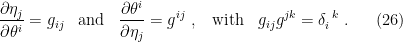
which follows from the definition ${\langle\nabla_{\partial_i}\partial_j,\partial_k\rangle=\Gamma_{ij,k}}$ , and similarly for ${\nabla^*}$ , with basis vectors ${Z=\partial_i}$ etc. Given a metric ${g}$ and connection ${\nabla}$ on ${S}$ , the dual connection ${\nabla^*}$ is generally unique, and satisfies ${(\nabla^*)^*=\nabla}$ . Additionally, the combination ${(\nabla+\nabla^*)/2}$ is metric. Conversely, one immediately sees that the condition for ${\nabla}$ to be metric is that ${\nabla^*=\nabla}$ , and in this sense dual connections simply constitute a more general class thereof.

In particular, ${\nabla^{(\alpha)}}$ and ${\nabla^{(-\alpha)}}$ are dual with respect to the Fisher metric. This follows readily from the general expressions for the ${\alpha}$ -connection developed in section 2.6, which we’ve skipped over here. Suffice to say the framework of ${(\pm1)}$ -connection admits a straightforward extension to arbitrary ${\alpha}$ .

The significance of dual connections is neatly illustrated by considering the parallel transport along a curve ${\gamma}$ from ${T_pS\rightarrow T_qS}$ with respect to ${\nabla}$ and ${\nabla^*}$ , respectively denoted ${\Pi_\gamma}$ and ${\Pi_\gamma^*}$ . As mentioned in the previous post, general ${\alpha}$ connections are not metric; but the dual structure allows one to generalize the notion of preservation of the inner product along a curve, namely:

$\displaystyle \langle\Pi_\gamma X,\Pi_\gamma^* Y\rangle_q=\langle X,Y\rangle_p~\quad\forall X,Y\in T_pS~. \ \ \ \ \ (14)$

And furthermore, the relationship between ${\Pi_\gamma}$ and ${\Pi_\gamma^*}$ is completely fixed by this condition.

Divergences

The duality structure of statistical manifolds facilitates the introduction of a distance-like measure ${D}$ , which enables us to compute something like a geometrical distance between distributions. In particular, we shall define a smooth function ${D(\cdot||\cdot):S\times S\rightarrow\mathbb{R}}$ such that ${D(p||q)\geq0\;\;\forall p,q\in S}$ , with equality iff ${p=q}$ . While this provides a measure of the separation between ${p}$ and ${q}$ , it is asymmetric and does not satisfy the triangle inequality, and hence fails the conditions for a distance function. However, if ${D}$ further satisfies

$\displaystyle \begin{aligned} D(\partial_i||\cdot)=D&(\cdot||\partial_i)=0~,\\ D(\partial_i\partial_j||\cdot)=D(\cdot||\partial_i\partial_j)&=-D(\partial_i||\partial_j)\equiv g_{ij}^{(D)}~, \end{aligned} \ \ \ \ \ (15)$

where ${[g_{ij}^{(D)}]}$ is a positive definite matrix everywhere on ${S}$ , then ${D}$ is a divergence or contrast function on ${S}$ . Note that a divergence uniquely defines a Riemannian metric ${g^{(D)}=\langle\cdot,\cdot\rangle^{(D)}}$ via

$\displaystyle \langle X,Y\rangle^{(D)}=-D(X||Y)~, \ \ \ \ \ (16)$

i.e., ${\langle\partial_i,\partial_j\rangle^{(D)}=g_{ij}^{(D)}}$ . We can also define an affine connection ${\nabla^{(D)}}$ associated with this divergence, via the coefficients ${\Gamma_{ij,k}^{(D)}}$

$\displaystyle \Gamma_{ij,k}^{(D)}=-D(\partial_i\partial_j||\partial_k)\;\;\iff\;\; \langle\nabla_X^{(D)}Y,Z\rangle^{(D)}=-D(XY||Z)~. \ \ \ \ \ (17)$

Similarly, we define the dual ${D^*(p||q)\equiv D(q||p)}$ , from which we have ${g^{(D^*)}=g^{(D)}}$ and ${\Gamma_{ij,k}^{(D^*)}=-D(\partial_k||\partial_i\partial_j)}$ . Thus we have that ${\nabla^{(D)}}$ and ${\nabla^{(D^*)}}$ are dual with respect to ${g^{(D)}}$ . In fact, any dual structure ${(g,\nabla,\nabla^*)}$ is naturally induced from a divergence!

Of course, the above is quite general: there are infinitely many different divergences one could define on a manifold. Henceforth we shall specify to a particularly important class for statistical models, known as the f-divergence:

$\displaystyle D_f(p||q)\equiv\int\!\mathrm{d} x\,p(x)f\!\left(\frac{q(x)}{p(x)}\right)~, \ \ \ \ \ (18)$

where ${f(u)}$ is an arbitrary convex function on ${0<u\in\mathbb{R}}$ with ${f(1)=0}$ . The f-divergence satisfies a number of important properties (see page 56), chief of which is monotonicity under arbitrary probability transition functions. That is, let ${x\in\mathcal{X}}$ be randomly transformed into ${y\in\mathcal{Y}}$ with probability ${\kappa(y|x)\geq0}$ , with ${\int\!\mathrm{d} y\,\kappa(y|x)=1\;\;\forall x}$ . This maps distributions ${p(x),q(x)}$ to ${p_\kappa(y),q_\kappa(y)}$ , respectively. Monotonicity of the f-divergence is then the statement that

$\displaystyle D_f(p||q)\geq D_f(p_\kappa||q_\kappa)~. \ \ \ \ \ (19)$

Spoiler alert: this will surface again in the form of monotonicity of relative entropy below! Note that ${\kappa}$ is a generalization of the deterministic mapping induced by ${F:\mathcal{X}\rightarrow\mathcal{Y}}$ in the previous post, which corresponds to ${\kappa(y,x)=\delta_{F(x)}y}$ . Consequently, the equality is saturated iff ${\kappa}$ is induced from a sufficient statistic, for which ${p_\kappa(x|y)=q_\kappa(x|y)\;\;\forall x,y}$ .

Within this still-broad class of f-divergences, one finds the ${\alpha}$ -divergence ${D^{(\alpha)}=D_{f^{(\alpha)}}}$ , defined for all ${\alpha\in\mathbb{R}}$ via

$\displaystyle f^{(\alpha)}(u)=\begin{cases} \frac{4}{1-\alpha^2}\left(1-u^{(1+\alpha)/2}\right) \;\; & \alpha\neq\pm1\\ u\ln u & \alpha=1\\ -\ln u & \alpha=-1 \end{cases}~, \ \ \ \ \ (20)$

which yields, for ${\alpha\neq\pm1}$ ,

$\displaystyle D^{(\alpha)}(p||q)=\frac{4}{1-\alpha^2}\left(1-\int\!\mathrm{d} x\,p(x)^{\frac{1-\alpha}{2}}q(x)^{\frac{1+\alpha}{2}}\right)~, \ \ \ \ \ (21)$

and, for ${\alpha=\pm1}$ ,

$\displaystyle D^{(-1)}(p||q)=D^{(1)}(q||p)=\int\!\mathrm{d} x\,p(x)\ln\frac{p(x)}{q(x)}~. \ \ \ \ \ (22)$

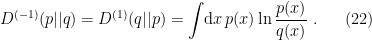
Of course, this last is none other than the relative entropy or Kullback-Leibler divergence!

The ${\alpha}$ -divergence ${D^{(\alpha)}}$ is so named because it naturally induces the dual structure ${(g,\nabla^{(\alpha)},\nabla^{(-\alpha)})}$ , i.e., the Fisher metric and (dual) ${\alpha}$ -connections. Let us now explore this duality in more detail, which will lead us to a deeper appreciation for the divergence ${D}$ .

Dually flat spaces

Suppose that, in a dual structure ${(g,\nabla,\nabla^*)}$ , both connections are symmetric, as is the case for ${\alpha}$ -connections. This implies that ${\alpha}$ -flatness and ${(-\alpha)}$ -flatness of ${S}$ are equivalent. In particular, we’ve seen that e-families are 1-flat, and m-families are ${(-1)}$ -flat, but the above implies that in fact they are both ${(\pm1)}$ -flat. In general, if both duals ${\nabla}$ and ${\nabla^*}$ are flat, we call ${(S,g,\nabla,\nabla^*)}$ a dually flat space. Such spaces have a number of properties that are closely related to various concepts in statistics.

By definition, there exist ${\nabla}$ -affine and ${\nabla^*}$ -affine coordinate systems ${[\theta^i]}$ and ${[\eta_j]}$ , respectively, in which vector fields are denoted ${\partial_i\equiv\frac{\partial}{\partial\theta^i}}$ and ${\partial_j\equiv\frac{\partial}{\partial\eta_j}}$ . Since both ${\partial_i}$ and ${\partial^j}$ are flat, the condition on parallel transport (14) implies that ${\langle\partial_i,\partial^j\rangle}$ is in fact constant on ${S}$ . Furthermore, given ${[\theta^i]}$ , affine transformations allow us to choose the dual coordinate system ${[\eta^j]}$ such that

$\displaystyle \langle\partial_i,\partial^j\rangle=\delta_i^{~j}~. \ \ \ \ \ (23)$

Coordinate systems which satisfy this requirement are called mutually dual. Such coordinate systems are special to dually flat spaces, and do not exist for general Riemannian manifolds; conversely, if one finds such coordinates for a Riemannian manifold ${(S,g)}$ , then the connections ${\nabla}$ and ${\nabla^*}$ for which they are affine are uniquely determined, and ${(S,g,\nabla,\nabla^*)}$ is a dually flat space.

A quick remark on notation: we shall denote the components of the metric ${g}$ with respect to ${[\theta^i]}$ and ${[\eta_j]}$ by

$\displaystyle g_{ij}\equiv\langle\partial_i,\partial_j\rangle\;\;\mathrm{and}\;\; g^{ij}\equiv\langle\partial^i,\partial^j\rangle~. \ \ \ \ \ (24)$

Coordinate transformations between them are given by the usual expressions,

$\displaystyle \partial^j=(\partial^j\theta^i)\partial_i\;\;\mathrm{and}\;\; \partial_i=(\partial_i\eta_j)\partial^j~. \ \ \ \ \ (25)$

In conjunction with (23), we therefore have

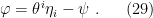
$\displaystyle \frac{\partial\eta_j}{\partial\theta^i}=g_{ij}\;\;\;\mathrm{and}\;\;\; \frac{\partial\theta^i}{\partial\eta_j}=g^{ij}~,\;\;\;\mathrm{with}\;\;\; g_{ij}g^{jk}=\delta_i^{~k}~. \ \ \ \ \ (26)$

We may now introduce the potentials, which will prove useful below. At a mathematical level, these allow us to define the Legendre transformation that explicitly relates the dual coordinate systems ${[\theta^i]}$ and ${[\eta_j]}$ . Consider a function ${\psi:S\rightarrow\mathbb{R}}$ that satisfies the following partial differential equation:

$\displaystyle \partial_i\psi=\eta_i\qquad\iff\qquad\mathrm{d}\psi=\eta_i\mathrm{d}\theta^i~. \ \ \ \ \ (27)$

From the coordinate expressions above, ${\partial_i\partial_j\psi=g_{ij}}$ , and hence the second derivatives of ${\psi}$ comprise a positive definite matrix. Hence ${\psi}$ is a strictly convex function of ${[\theta^i]}$ . Similarly, define ${\varphi}$ such that

$\displaystyle \partial^i\varphi=\theta^i\qquad\iff\qquad\mathrm{d}\varphi=\theta^i\mathrm{d}\eta_i~, \ \ \ \ \ (28)$

which is a strictly convex function of ${[\eta_j]}$ , since ${\partial^i\partial^j\varphi=g^{ij}}$ . These two functions are related via

$\displaystyle \varphi=\theta^i\eta_i-\psi~. \ \ \ \ \ (29)$

To see this, simply take the differential ${\mathrm{d}\varphi=\mathrm{d}\theta^i\eta_i+\theta^i\mathrm{d}\eta_i-\mathrm{d}\psi}$ , whereupon substituting in (27) one recovers (28). Now, the form of (29) — equivalently, the pair (27) and (28) — suggests that ${[\theta^i]}$ , ${[\eta_j]}$ form a conjugate pair of coordinates for the functions ${\psi}$ , ${\varphi}$ in the context of Legendre transforms. However, (29) does not quite suffice to define the Legendre transform, since we must remove the ${\theta}$ dependence on the right-hand side in order for it to be uniquely invertible. Note that (strict) convexity is important here, since this implies a 1:1 map between a function and its first derivative, which in turn enables one — via the Legendre transform — to express all the information about a function in terms of its derivatives instead. By analogy with Fourier or Laplace transforms, this may lead to deeper mathematical/physical insight, or simple convenience, depending on the application. Hence, since we’re dealing with strictly convex functions, we define the Legendre transforms

$\displaystyle \varphi(q)=\mathrm{sup}_{p\in S}\left[\theta^i(p)\eta_i(q)-\psi(p)\right]\quad\mathrm{and}\quad \psi(p)=\mathrm{sup}_{q\in S}\left[\theta^i(p)\eta_i(q)-\varphi(q)\right]~. \ \ \ \ \ (30)$

Thus we see that the dual/conjugate coordinate systems ${[\theta^i]}$ and ${[\eta_j]}$ are related by the Legendre transform given in terms of the potentials ${\psi}$ and ${\varphi}$ , which provides another explanation for the name.

Incidentally, in addition to the compact expressions for the metric above, namely

$\displaystyle \partial_i\partial_j\psi=g_{ij}\quad\mathrm{and}\quad \partial^i\partial^j\varphi=g^{ij}~, \ \ \ \ \ (31)$

the potentials also enable one to neatly express the connection coefficients as

$\displaystyle \Gamma_{ij,k}^*\equiv\langle\nabla_{\partial_i}^*\partial_j,\partial_k\rangle=\partial_i\partial_j\partial_k\psi\quad\mathrm{and}\quad \Gamma^{ij,k}\equiv\langle\nabla_{\partial^i}\partial^j,\partial^k\rangle=\partial^i\partial^j\partial^k\varphi~. \ \ \ \ \ (32)$

Now, we mentioned earlier that any divergence induces a (torsion-free) dual structure, and vice-versa. But this map is not bijective; rather, a given dual structure admits infinitely many divergences. In the case of dually flat spaces however, the potentials defined above allow us to introduce a canonical divergence which is in some sense unique, namely

$\displaystyle D(p||q)\equiv\psi(p)+\varphi(q)-\theta^i(p)\eta_i(q)~, \ \ \ \ \ (33)$

which of course satisfies ${D(p||q)\geq0}$ , with equality iff ${p=q}$ . To see that ${D}$ is a divergence which induces the metric ${g}$ , observe that

$\displaystyle D\left((\partial_i\partial_j)p||q\right)=g_{ij}(p)\quad\mathrm{and}\quad D\left(p||(\partial^i\partial^j)q\right)=g^{ij}(q)~, \ \ \ \ \ (34)$

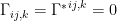which further implies ${\nabla=\nabla^{(D)}}$ and ${\nabla^*=\nabla^{(D^*)}}$ with ${\Gamma_{ij,k}={\Gamma^*}^{ij,k}=0}$ due to the ${\nabla}$ -, resp. ${\nabla^*}$ -affinity of ${[\theta^i]}$ , ${[\eta_j]}$ , where the dual divergence is ${D^*(p||q)=D(q||p)}$ .

Generic properties of such canonical divergences are examined in section 3.4. Instead however, I’m going to close this post by jumping ahead to 3.5, which connects this discussion back to the e- and m-families and associated ${(\pm1)}$ -connections we spent so much time on above.

Dual structure of exponential families

Recall that an exponential family consists of distributions of the form

$\displaystyle p(x;\theta)=\exp\left[C(x)+\theta^iF_i(x)-\psi(\theta)\right]~, \ \ \ \ \ (35)$

where the canonical parameters ${[\theta^i]}$ constitute a 1-affine coordinate system. The notation ${\psi}$ here was not chosen arbitrarily, but is in fact precisely the potential introduced above. This is a rather elegant fact that ties together some fundamental notions from statistics with the existence of the dual coordinates ${[\eta_i]}$ . Suppose we didn’t know that ${\eta}$ is the dual coordinate to ${\theta}$ , and simply defined

$\displaystyle \eta_i=\eta_i(\theta)\equiv E_\theta[F_i]=\int\!\mathrm{d} x\,F_i(x)p(x;\theta)~. \ \ \ \ \ (36)$

Then it follows that

$\displaystyle 0=E_\theta[\partial_i\ell_\theta]=E_\theta[F_i(x)-\partial_i\psi(\theta)]\;\;\implies\;\; \eta_i=\partial_i\psi~. \ \ \ \ \ (37)$

Additionally, the expression of the metric in the form ${g_{ij}(\theta)=-E_\theta[\partial_i\partial_j\ell_\theta]}$ implies that for an exponential family, ${\partial_i\partial_j\psi=g_{ij}}$ . Thus (0.36) suffices to identify ${\eta}$ as the conjugate parameter to ${\theta}$ with respect to the Legendre potential ${\psi}$ . From the discussion above, this implies that ${[\eta_i]}$ is a ${(-1)}$ -affine coordinate system dual to ${[\theta^i]}$ . Given the form of (0.36), ${[\eta_i]}$ are sometimes also referred to as the expectation parameters.

It is a trivial exercise to work out ${\eta_1}$ and ${\eta_2}$ for the example of the normal distribution in the previous post. A more interesting example is the case when ${\mathcal{X}}$ is a finite set, whence ${\mathcal{P}(\mathcal{X})}$ is identified with the parameters:

$\displaystyle \begin{aligned} \mathcal{X}=&\{x_0,\ldots,x_n\}~,\qquad \Xi=\left\{[\xi^i]\,\Big|\,\xi^i>0\;\;\forall i~,\;\;\sum_{i=1}^n\xi^i<1\right\}\\ &p(x_i;\xi)=\begin{cases} \xi^i & 1\leq i\leq n \\ 1-\sum_{i=1}^n\xi^i\quad & i=0 \end{cases}~. \end{aligned} \ \ \ \ \ (38)$

(This is introduced as example 2.4 on page 27, and resurfaces as example 2.8 on page 35 and example 3.4 on page 66). Expressing this as an exponential family of the form (0.35) implies the parameter identifications

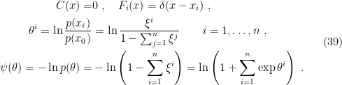
$\displaystyle \begin{aligned} C(x)=&0~,\quad F_i(x)=\delta(x-x_i)~,\\ \theta^i=\ln\frac{p(x_i)}{p(x_0)}&=\ln\frac{\xi^i}{1-\sum\nolimits_{j=1}^n\xi^j}\qquad i=1,\ldots,n~,\\ \psi(\theta)=-\ln p(\theta)=&-\ln\left(1-\sum_{i=1}^n\xi^i\right)=\ln\left(1+\sum_{i=1}^n\exp\theta^i\right)~. \end{aligned} \ \ \ \ \ (39)$

Then the dual coordinates ${[\eta_i]}$ are simply given by the parameters themselves:

$\displaystyle \eta_i=p(x_i)=\xi^i=\frac{\exp\theta^i}{1+\sum_{j=1}^n\exp\theta^j}~. \ \ \ \ \ (40)$

Therefore, the dual potential (29) is

$\displaystyle \varphi(\theta)=E_\theta[\ln p_\theta-C]=-H(p_\theta)-E_\theta[C]~, \ \ \ \ \ (41)$

where ${H(p)\equiv-\int\!\mathrm{d} x\,p(x)\ln p(x)}$ is the entropy!

Finally, I promised you some statistical notions, which requires the introduction of one more concept, namely that of an estimator. Suppose that some data ${x}$ is generated according to some unknown probability distribution ${p_\xi}$ . We wish to consider the problem of estimating the unknown parameter ${\xi}$ by some function ${\hat\xi(x)}$ of the data ${x}$ . The mapping ${[\hat\xi^i]:\mathcal{X}\rightarrow\mathbb{R}^n}$ is called an estimator. Furthermore, ${\hat\xi}$ is an unbiased estimator if

$\displaystyle E_\xi[\hat\xi(X)]=\xi\quad\forall\xi\in\Xi~, \ \ \ \ \ (42)$

which is the statement that the expectation value of ${\hat\xi}$ does not depend on the data itself. The mean-squared error of such an estimator may be expressed via the variance-covariance matrix ${V_\xi[\hat\xi]=[v_\xi^{ij}]}$ , whose elements are defined via

$\displaystyle v_\xi^{ij}\equiv E_\xi\left[(\hat\xi^i(X)-\xi^i)(\hat\xi^j(X)-\xi^j)\right]~. \ \ \ \ \ (43)$

Lastly, the Cramér-Rao inequality (Theorem 2.2) states that the variance-covariance matrix of an unbiased estimator satisfies

$\displaystyle V_\xi[\hat\xi]\geq G(\xi)^{-1}~, \ \ \ \ \ (44)$

i.e., the difference ${V_\xi[\hat\xi]-G(\xi)^{-1}}$ is a positive semidefinite matrix. An unbiased estimator ${\hat\xi}$ which saturates this inequality for all ${\xi}$ is an efficient estimator, which means it has the minimum variance among all unbiased estimators (note however that the converse is not always true).

Efficient estimators do not exist for arbitrary coordinates ${\xi}$ . Rather, a necessary and sufficient condition for a model ${S=\{p_\xi\}}$ to have an efficient estimator is that ${S}$ be an exponential family, for which ${\xi}$ is m-affine (Theorem 3.12).

To illustrate this, let us now regard ${F_i}$ as an estimator for the parameter ${\eta_i}$ , which we shall henceforth denote ${\hat\eta_i(x)=F_i(x)}$ to make contact with the notation just introduced. Then the condition (0.36) implies that ${\hat\eta}$ is in fact an unbiased estimator for ${\eta}$ . Furthermore, since the Fisher information matrix can be expressed in terms of ${F}$ and ${\eta}$ as

$\displaystyle g_{ij}(\theta)=E_\theta[(F_i-\eta_i)(F_j-\eta_j)]~, \ \ \ \ \ (45)$

it follows that ${V_\eta[\hat\eta]=G=[g_{ij}]}$ , and hence ${\hat\eta}$ is an efficient estimator for the (m-affine) coordinate system ${\eta}$ .

The above is of course only a superficial hint of the deeper connections between information geometry and statistics (which was, after all, the prime impetus for the former’s development), but already suggests interesting mathematical utility for such problems as maximum likelihood estimation (MLE), and machine learning in general. Alas, that’s a topic for another post.

As a final comment: everything I’ve said so far is for classical probability distributions, but much of this machinery can be extended to quantum mechanics as well (insofar as the latter can be viewed as an extension of probability theory). Quantum information geometry is briefly introduced in chapter 7, and I hope to return to it in part 3 of this series soon.

2 Responses to Information geometry (part 2/3)

JG says:

May 25, 2020 at 10:24 pm

These three posts are a wonderful review of information geometry! Thanks so much!

A quick note, in equation (30), I think the RHS of the left expression should have a psi instead of a phi.

LikeLike

- irreverentmind says:
  
  May 28, 2020 at 12:23 pm
  
  Thanks JG, I’m delighted you found them helpful!
  
  Whoops, indeed that’s a typo; fixed now. Thanks for the catch!
  
  LikeLike