Information geometry is a rather interesting fusion of statistics and differential geometry, in which a statistical model is endowed with the structure of a Riemannian manifold. Each point on the manifold corresponds to a probability distribution function, and the metric is governed by the underlying properties thereof. It may have many interesting applications to (quantum) information theory, complexity, machine learning, and theoretical neuroscience, among other fields. The canonical reference is Methods of Information Geometry by Shun-ichi Amari and Hiroshi Nagaoka, originally published in Japanese in 1993, and translated into English in 2000. The English version also contains several new topics/sections, and thus should probably be considered as a “second edition” (incidentally, any page numbers given below refer to this version). This is a beautiful book, which develops the concepts in a concise yet pedagogical manner. The posts in this three-part series are merely the notes I made while studying it, and aren’t intended to provide more than a brief summary of what I deemed the salient aspects.
Chapter 1 provides a self-contained introduction to differential geometry which — as the authors amusingly allude — is far more accessible (dare I say practical) than the typical mathematician’s treatise on the subject. Since this is familiar material, I’ll skip ahead to chapter 2, and simply recall necessary formulas/notation as needed.
Chapter 2 introduces the basic geometric structure of statistical models. First, some notation: a probability distribution is a function  which satisfies
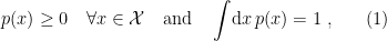
where  . If
. If  is a discrete set (which may have either finite or countably infinite cardinality), then the integral is instead a sum. Each
  may be parametrized by
  real-valued variables
 ![{\xi=[\xi^i]=[\xi^1,\ldots,\xi^n]}](https://s0.wp.com/latex.php?latex=%7B%5Cxi%3D%5B%5Cxi%5Ei%5D%3D%5B%5Cxi%5E1%2C%5Cldots%2C%5Cxi%5En%5D%7D&bg=ffffff&fg=000000&s=0&c=20201002) , such that the family
, such that the family  of probability distributions on is
![\displaystyle S=\{p_\xi=p(x;\xi)\,|\,\xi=[\xi^i]\in\Xi\}~, \ \ \ \ \ (2)](https://s0.wp.com/latex.php?latex=%5Cdisplaystyle+S%3D%5C%7Bp_%5Cxi%3Dp%28x%3B%5Cxi%29%5C%2C%7C%5C%2C%5Cxi%3D%5B%5Cxi%5Ei%5D%5Cin%5CXi%5C%7D%7E%2C+%5C+%5C+%5C+%5C+%5C+%282%29&bg=ffffff&fg=000000&s=0&c=20201002)
where  and
and  is injective (so that the reverse mapping, from probability distributions to the coordinates
  is a function). Such an is referred to as an -dimensional statistical model, or simply model on , sometimes abbreviated
  . Note that I referred to as the coordinates above: we will assume that the map
  provided by is
  , so that we may take derivatives with respect to the parameters, e.g.,
  , where
  . Additionally, we assume that the order of differentiation and integration may be freely exchanged; an important consequence of this is that

which we will use below. Finally, we assume that the support of the distribution  is independent of (that is, does not vary with) , and hence may redefine
  for simplicity. Thus, the model is a subset of

Considering parametrizations which are diffeomorphic to one another to be equivalent then elevates to a statistical manifold. (In this context, we shall sometimes conflate the distribution  with the coordinate , and speak of the “point ”, etc).
As a concrete example, consider the normal distribution:
![\displaystyle p(x;\xi)=\frac{1}{\sqrt{2\pi}\sigma}\exp\left[-\frac{\left(x-\mu\right)^2}{2\sigma^2}\right]~. \ \ \ \ \ (5)](https://s0.wp.com/latex.php?latex=%5Cdisplaystyle+p%28x%3B%5Cxi%29%3D%5Cfrac%7B1%7D%7B%5Csqrt%7B2%5Cpi%7D%5Csigma%7D%5Cexp%5Cleft%5B-%5Cfrac%7B%5Cleft%28x-%5Cmu%5Cright%29%5E2%7D%7B2%5Csigma%5E2%7D%5Cright%5D%7E.+%5C+%5C+%5C+%5C+%5C+%285%29&bg=ffffff&fg=000000&s=0&c=20201002)
In this case,
![\displaystyle \mathcal{X}=\mathbb{R}~,\;\;n=2,\;\;\xi=[\mu,\sigma],\;\;\Xi=\{[\mu,\sigma]\,|\,\mu\in\mathbb{R},\;\sigma\in\mathbb{R}^+\}~. \ \ \ \ \ (6)](https://s0.wp.com/latex.php?latex=%5Cdisplaystyle+%5Cmathcal%7BX%7D%3D%5Cmathbb%7BR%7D%7E%2C%5C%3B%5C%3Bn%3D2%2C%5C%3B%5C%3B%5Cxi%3D%5B%5Cmu%2C%5Csigma%5D%2C%5C%3B%5C%3B%5CXi%3D%5C%7B%5B%5Cmu%2C%5Csigma%5D%5C%2C%7C%5C%2C%5Cmu%5Cin%5Cmathbb%7BR%7D%2C%5C%3B%5Csigma%5Cin%5Cmathbb%7BR%7D%5E%2B%5C%7D%7E.+%5C+%5C+%5C+%5C+%5C+%286%29&bg=ffffff&fg=000000&s=0&c=20201002)
Other examples are given on page 27.
Fisher information metric
Now, given a model , the Fisher information matrix of at a point is the  matrix
 ![{G(\xi)=[g_{ij}(\xi)]}](https://s0.wp.com/latex.php?latex=%7BG%28%5Cxi%29%3D%5Bg_%7Bij%7D%28%5Cxi%29%5D%7D&bg=ffffff&fg=000000&s=0&c=20201002) , with elements
, with elements
![\displaystyle g_{ij}(\xi)\equiv E_\xi[\partial_i\ell_\xi\partial_j\ell_\xi] =\int\!\mathrm{d} x\,\partial_i\ell(x;\xi)\partial_j\ell(x;\xi)p(x;\xi)~, \ \ \ \ \ (7)](https://s0.wp.com/latex.php?latex=%5Cdisplaystyle+g_%7Bij%7D%28%5Cxi%29%5Cequiv+E_%5Cxi%5B%5Cpartial_i%5Cell_%5Cxi%5Cpartial_j%5Cell_%5Cxi%5D+%3D%5Cint%5C%21%5Cmathrm%7Bd%7D+x%5C%2C%5Cpartial_i%5Cell%28x%3B%5Cxi%29%5Cpartial_j%5Cell%28x%3B%5Cxi%29p%28x%3B%5Cxi%29%7E%2C+%5C+%5C+%5C+%5C+%5C+%287%29&bg=ffffff&fg=000000&s=0&c=20201002)
where

and the expectation  with respect to the distribution is defined as
![\displaystyle E_\xi[f]\equiv\int\!\mathrm{d} x\,f(x)p(x;\xi)~. \ \ \ \ \ (9)](https://s0.wp.com/latex.php?latex=%5Cdisplaystyle+E_%5Cxi%5Bf%5D%5Cequiv%5Cint%5C%21%5Cmathrm%7Bd%7D+x%5C%2Cf%28x%29p%28x%3B%5Cxi%29%7E.+%5C+%5C+%5C+%5C+%5C+%289%29&bg=ffffff&fg=000000&s=0&c=20201002)
Though the integral above diverges for some models, we shall assume that  is finite
  , and furthermore that
  is . Note that
  (i.e.,
  is symmetric). Additionally, while is in general positive semidefinite, we shall assume positive definiteness, which is equivalent to requiring that
  are linearly independent functions on . Lastly, observe that eq. (3) may be written
![\displaystyle E_\xi[\partial_i\ell_\xi]=0~. \ \ \ \ \ (10)](https://s0.wp.com/latex.php?latex=%5Cdisplaystyle+E_%5Cxi%5B%5Cpartial_i%5Cell_%5Cxi%5D%3D0%7E.+%5C+%5C+%5C+%5C+%5C+%2810%29&bg=ffffff&fg=000000&s=0&c=20201002)
Via integration by parts, this allows us to express the matrix elements in a useful alternative form:
![\displaystyle g_{ij}(\xi)=-E_\xi[\partial_i\partial_j\ell_\xi]~. \ \ \ \ \ (11)](https://s0.wp.com/latex.php?latex=%5Cdisplaystyle+g_%7Bij%7D%28%5Cxi%29%3D-E_%5Cxi%5B%5Cpartial_i%5Cpartial_j%5Cell_%5Cxi%5D%7E.+%5C+%5C+%5C+%5C+%5C+%2811%29&bg=ffffff&fg=000000&s=0&c=20201002)
The reason for the particular definition of the Fisher matrix above is that it provides a Riemannian metric on . Recall that a Riemannian metric  is a
is a  -tensor (that is, it maps points in to their inner product on the tangent space
  ) which is linear, symmetric, and positive definite (meaning
  , with equality iff
  ). In fact, in the natural basis of local coordinates
 ![{[\xi^i]}](https://s0.wp.com/latex.php?latex=%7B%5B%5Cxi%5Ei%5D%7D&bg=ffffff&fg=000000&s=0&c=20201002) , the Riemannian metric is uniquely determined by
, the Riemannian metric is uniquely determined by

whence  is called the Fisher metric. Since it’s positive definite, we may define the inverse metric
  corresponding to
  such that
  . Note that
  is invariant under coordinate transformations, since

and hence we may write
![\displaystyle \langle X,Y\rangle_\xi=E_\xi[(X\ell)(Y\ell)]\quad\forall X,Y\in T_\xi S~. \ \ \ \ \ (14)](https://s0.wp.com/latex.php?latex=%5Cdisplaystyle+%5Clangle+X%2CY%5Crangle_%5Cxi%3DE_%5Cxi%5B%28X%5Cell%29%28Y%5Cell%29%5D%5Cquad%5Cforall+X%2CY%5Cin+T_%5Cxi+S%7E.+%5C+%5C+%5C+%5C+%5C+%2814%29&bg=ffffff&fg=000000&s=0&c=20201002)
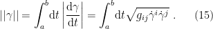
Recalling that  , the length of a curve
 ![{\gamma:[a,b]\rightarrow S}](https://s0.wp.com/latex.php?latex=%7B%5Cgamma%3A%5Ba%2Cb%5D%5Crightarrow+S%7D&bg=ffffff&fg=000000&s=0&c=20201002) with respect to g is then
with respect to g is then
But before we can properly speak of curves and distances, we must define a connection, which provides a means of parallel transporting vectors along the curve.
 -connections
In particular, we will be concerned with comparing elements of the tangent bundle, and hence we require a relation between the tangent spaces at different points in , i.e., an affine connection. To that end, let be an -dimensional model, and define the  functions
  which map each point to
![\displaystyle \left(\Gamma_{ij,k}^{(\alpha)}\right)_\xi\equiv E_\xi\left[\left(\partial_i\partial_j\ell_\xi+\frac{1-\alpha}{2}\partial_i\ell_\xi\partial_j\ell_\xi\right)\left(\partial_k\ell_\xi\right)\right]~, \ \ \ \ \ (16)](https://s0.wp.com/latex.php?latex=%5Cdisplaystyle+%5Cleft%28%5CGamma_%7Bij%2Ck%7D%5E%7B%28%5Calpha%29%7D%5Cright%29_%5Cxi%5Cequiv+E_%5Cxi%5Cleft%5B%5Cleft%28%5Cpartial_i%5Cpartial_j%5Cell_%5Cxi%2B%5Cfrac%7B1-%5Calpha%7D%7B2%7D%5Cpartial_i%5Cell_%5Cxi%5Cpartial_j%5Cell_%5Cxi%5Cright%29%5Cleft%28%5Cpartial_k%5Cell_%5Cxi%5Cright%29%5Cright%5D%7E%2C+%5C+%5C+%5C+%5C+%5C+%2816%29&bg=ffffff&fg=000000&s=0&c=20201002)
where  . This defines an affine connection
  on via

where  is the Fisher metric introduced above. is called the -connection, and accordingly terms like -flat, -affine, -parallel, etc. denote the corresponding notions with respect to this connection.
Let us pause to review some of the terminology from differential geometry above. Recall that the covariant derivative  may be expressed in local coordinates as

where  ,
,  are vectors in the tangent space. If these are basis vectors such that
  , then
  . The vector
  is said to be parallel with respect to the connection if
  , i.e.,
  ; equivalently, in local coordinates,

If all basis vectors are parallel with respect to a coordinate system , then the latter is an affine coordinate system for . Connections which admit such an affine parametrization are called flat (equivalently, one says that is flat with respect to ).
Now, with respect to a Riemannian metric , one defines  as above, namely
  . Note that this defines a symmetric connection, i.e.,
  . If, in addition, satisfies

then is a metric connection with respect to . (This is basically a statement about linearity, since affine transformations are linear). This implies that

In other words, under a metric connection, parallel transport of two vectors preserves the inner product, hence their significance in Riemannian geometry. Any connection which is both metric and symmetric is Riemannian, of which there are generically an infinite number. However, the natural metrics on statistical manifolds are generically non-metric! Indeed, since
![\displaystyle \begin{aligned} \partial_kg_{ij}&=\partial_kE_\xi[\partial_i\ell_\xi\partial_j\ell_\xi]\\ &=E_\xi[\left(\partial_k\partial_i\ell_\xi\right)\left(\partial_j\ell_\xi\right)]+E_\xi[\left(\partial_i\ell_\xi\right)\left(\partial_k\partial_j\ell_\xi\right)]+E_\xi[\left(\partial_i\ell_\xi\right)\left(\partial_j\ell_\xi\right)\left(\partial_k\ell_\xi\right)]\\ &=\Gamma_{ki,j}^{(0)}+\Gamma_{kj,i}^{(0)}~, \end{aligned} \ \ \ \ \ (22)](https://s0.wp.com/latex.php?latex=%5Cdisplaystyle+%5Cbegin%7Baligned%7D+%5Cpartial_kg_%7Bij%7D%26%3D%5Cpartial_kE_%5Cxi%5B%5Cpartial_i%5Cell_%5Cxi%5Cpartial_j%5Cell_%5Cxi%5D%5C%5C+%26%3DE_%5Cxi%5B%5Cleft%28%5Cpartial_k%5Cpartial_i%5Cell_%5Cxi%5Cright%29%5Cleft%28%5Cpartial_j%5Cell_%5Cxi%5Cright%29%5D%2BE_%5Cxi%5B%5Cleft%28%5Cpartial_i%5Cell_%5Cxi%5Cright%29%5Cleft%28%5Cpartial_k%5Cpartial_j%5Cell_%5Cxi%5Cright%29%5D%2BE_%5Cxi%5B%5Cleft%28%5Cpartial_i%5Cell_%5Cxi%5Cright%29%5Cleft%28%5Cpartial_j%5Cell_%5Cxi%5Cright%29%5Cleft%28%5Cpartial_k%5Cell_%5Cxi%5Cright%29%5D%5C%5C+%26%3D%5CGamma_%7Bki%2Cj%7D%5E%7B%280%29%7D%2B%5CGamma_%7Bkj%2Ci%7D%5E%7B%280%29%7D%7E%2C+%5Cend%7Baligned%7D+%5C+%5C+%5C+%5C+%5C+%2822%29&bg=ffffff&fg=000000&s=0&c=20201002)
only the special case  defines a Riemannian connection
  with respect to the Fisher metric (though observe that is symmetric for any value of ). While this may seem strange from a physics perspective, where preserving the inner product is of prime importance, there’s nothing mathematically pathological about it. Indeed, the more relevant condition — which we’ll see below — is that every point on the manifold have an interpretation as a probability distribution.
Two neat relationships between different -connections are worth noting. First, for any  , we have
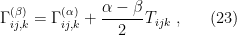
where  (not to be confused with the unrelated torsion tensor) is a covariant symmetric tensor which maps a point to
![\displaystyle \left(T_{ijk}\right)_\xi\equiv E_\xi[\partial_i\ell_\xi\partial_j\ell_\xi\partial_k\ell_\xi]~. \ \ \ \ \ (24)](https://s0.wp.com/latex.php?latex=%5Cdisplaystyle+%5Cleft%28T_%7Bijk%7D%5Cright%29_%5Cxi%5Cequiv+E_%5Cxi%5B%5Cpartial_i%5Cell_%5Cxi%5Cpartial_j%5Cell_%5Cxi%5Cpartial_k%5Cell_%5Cxi%5D%7E.+%5C+%5C+%5C+%5C+%5C+%2824%29&bg=ffffff&fg=000000&s=0&c=20201002)
Second, the -connection may be decomposed as

Within this infinite class of connections,  play a central role in information geometry, and are closely related to an interesting duality structure on the geometry of
  . We shall give a low-level introduction to the relevant representations of here, and postpone a more elegant derivation based on different embeddings of
  in
in  in the next post. In particular, we’ll define the so-called exponential and mixed families, which are intimately related to the
  – and
– and  -connections, respectively.
Exponential families
Suppose that an -dimensional model  can be expressed in terms of
  functions
  on and a function
  on
on  as
as
![\displaystyle p(x;\theta)=\exp\left[C(x)+\theta^iF_i(x)-\psi(\theta)\right]~, \ \ \ \ \ (26)](https://s0.wp.com/latex.php?latex=%5Cdisplaystyle+p%28x%3B%5Ctheta%29%3D%5Cexp%5Cleft%5BC%28x%29%2B%5Ctheta%5EiF_i%28x%29-%5Cpsi%28%5Ctheta%29%5Cright%5D%7E%2C+%5C+%5C+%5C+%5C+%5C+%2826%29&bg=ffffff&fg=000000&s=0&c=20201002)
where we’ve employed Einstein’s summation notation for the sum over  from to . Then is an exponential family, and
 ![{[\theta^i]}](https://s0.wp.com/latex.php?latex=%7B%5B%5Ctheta%5Ei%5D%7D&bg=ffffff&fg=000000&s=0&c=20201002) are its natural or canonical parameters. The normalization condition
are its natural or canonical parameters. The normalization condition  implies that
![\displaystyle \psi(\theta)=\log\int\!\mathrm{d} x\,\exp\left[C(x)+\theta^iF_i(x)\right]~. \ \ \ \ \ (27)](https://s0.wp.com/latex.php?latex=%5Cdisplaystyle+%5Cpsi%28%5Ctheta%29%3D%5Clog%5Cint%5C%21%5Cmathrm%7Bd%7D+x%5C%2C%5Cexp%5Cleft%5BC%28x%29%2B%5Ctheta%5EiF_i%28x%29%5Cright%5D%7E.+%5C+%5C+%5C+%5C+%5C+%2827%29&bg=ffffff&fg=000000&s=0&c=20201002)
This provides a parametrization  , which is
  if and only if the functions are linearly independent (which we shall assume henceforth). Many important probabilistic models fall into this class, including all those referenced on page 27 above. The normal distribution (5), for instance, yields

The canonical coordinates are natural insofar as they provide a -affine coordinate system, with respect to which is -flat. To see this, observe that

where keep in mind that  denotes the derivative with respect to
  , not
, not  ! This implies that
![\displaystyle \left(\Gamma_{ij,k}^{(1)}\right)_\theta=E_\theta[\left(\partial_i\partial_j\ell_\theta\right)\left(\partial_k\ell_\theta\right)] =-\partial_i\partial_j\psi(\theta)E_\theta[\partial_k\ell_\theta]=0~. \ \ \ \ \ (30)](https://s0.wp.com/latex.php?latex=%5Cdisplaystyle+%5Cleft%28%5CGamma_%7Bij%2Ck%7D%5E%7B%281%29%7D%5Cright%29_%5Ctheta%3DE_%5Ctheta%5B%5Cleft%28%5Cpartial_i%5Cpartial_j%5Cell_%5Ctheta%5Cright%29%5Cleft%28%5Cpartial_k%5Cell_%5Ctheta%5Cright%29%5D+%3D-%5Cpartial_i%5Cpartial_j%5Cpsi%28%5Ctheta%29E_%5Ctheta%5B%5Cpartial_k%5Cell_%5Ctheta%5D%3D0%7E.+%5C+%5C+%5C+%5C+%5C+%2830%29&bg=ffffff&fg=000000&s=0&c=20201002)
Therefore, exponential families admit a canonical parametrization in terms of a -affine coordinate system , with respect to which is -flat. The associated affine connection is called the exponential connection, and is denoted  .
.
Mixed families
Now consider the case in which can be expressed as

i.e., is an affine subspace of  . In this case is called a
  , with mixture parameters . Note that itself is a mixture family if is infinite. The name arises from the fact that elements in this family admit a representative form as a mixture of probability distributions
  ,
,
![\displaystyle p(x;\theta)=\theta^ip_i(x)+\left(1-\sum_{i=1}^n\theta^i\right)p_0(x) =p_0(x)+\sum_{i=1}^n\theta^i\left[p_i(x)-p_0(x)\right]~, \ \ \ \ \ (32)](https://s0.wp.com/latex.php?latex=%5Cdisplaystyle+p%28x%3B%5Ctheta%29%3D%5Ctheta%5Eip_i%28x%29%2B%5Cleft%281-%5Csum_%7Bi%3D1%7D%5En%5Ctheta%5Ei%5Cright%29p_0%28x%29+%3Dp_0%28x%29%2B%5Csum_%7Bi%3D1%7D%5En%5Ctheta%5Ei%5Cleft%5Bp_i%28x%29-p_0%28x%29%5Cright%5D%7E%2C+%5C+%5C+%5C+%5C+%5C+%2832%29&bg=ffffff&fg=000000&s=0&c=20201002)
(i.e.,  and
and  ), where
  and
and  . For a mixture family, we have

which implies that

Therefore, a mixture family admits a parametrization in terms of a -affine coordinate system , with respect to which is -flat. The associated affine connection is called the mixture connection, denoted  .
.
In the next post, when we discuss the geometrical structure in more detail, we shall see that are dual connections, which has many interesting consequences.
Why is Fisher special?
As noted above, a given manifold admits infinitely many distinct Riemannian metrics and affine connections. However, a statistical manifold has the property that every point is a probability distribution, which singles out the Fisher metric and -connection as unique. To formalize this notion, we must first introduce the concept of a sufficient statistic.
Let  be a map which takes random variables
  to
to  . Given the distribution
  of , this results in the distribution
  on . We then define

where  , and
, and  is the delta function at the point
  , such that
  ,
,

In other words, the delta function picks out the value of such that  . The above implies that
  is the conditional probability of the event
  , given
  (cf. the familiar definition
  ). If
). If  is independent of , then is called a sufficient statistic for . In this case, we may write

i.e., the dependence of on is entirely encoded in the distribution  . Therefore, treating as the unknown distribution, whose parameter one wishes to estimate, it suffices to know only the value
  , hence the name. Formally, one says that is a sufficient statistic if and only if there exists functions
 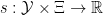 and
and  such that

The significance of this lies in the fact that the Fisher information metric satisfies a monotonicity relation under a generic map . This is detailed in Theorem 2.1 of Amari & Nagaoka, which states that given  with Fisher metric
  , and induced model
  with matrix
  , the difference
  is positive semidefinite, i.e.,
  , with equality if and only if is a sufficient statistic. Otherwise, for generic maps, the “information loss”
 ![{\Delta G(\xi)=[\Delta g_{ij}(\xi)]}](https://s0.wp.com/latex.php?latex=%7B%5CDelta+G%28%5Cxi%29%3D%5B%5CDelta+g_%7Bij%7D%28%5Cxi%29%5D%7D&bg=ffffff&fg=000000&s=0&c=20201002) that results from summarizing the data in
that results from summarizing the data in  is given by
![\displaystyle \Delta g_{ij}(\xi)=E_\xi[\partial_i\ln r(X;\xi)\partial_j\ln r(X;\xi)]~, \ \ \ \ \ (39)](https://s0.wp.com/latex.php?latex=%5Cdisplaystyle+%5CDelta+g_%7Bij%7D%28%5Cxi%29%3DE_%5Cxi%5B%5Cpartial_i%5Cln+r%28X%3B%5Cxi%29%5Cpartial_j%5Cln+r%28X%3B%5Cxi%29%5D%7E%2C+%5C+%5C+%5C+%5C+%5C+%2839%29&bg=ffffff&fg=000000&s=0&c=20201002)
which can be expressed in terms of the covariance with respect to the conditional distribution  . This theorem will be important later, when we discuss relative entropy.
Now, if is a sufficient statistic, then (37) implies that  . But this implies that , and by extension , are the same for both and
  . Therefore the Fisher metric and -connection are invariant with respect to the sufficient statistic . In the language above, this implies that there is no information loss associated with describing the original distribution by , i.e., that information is preserved under . Formally, this invariance is codified by the following two equations:

 , where the prime denotes the object on ,
  is the diffeomorphism from onto given by
  , and the pushforward
  is defined by
  .
.
The salient feature of the Fisher metric and -connection is that they are are uniquely characterized by this invariance! This is the thrust of Chentsov’s theorem (Theorem 2.6 in Amari & Nagaoka). Strictly speaking, the proof of this theorem relies on finiteness of , but — depending on the level of rigour one demands — it is possible to extend this to infinite models via a limiting procedure in which one considers increasingly fine-grained subsets of . A similar subtlety will arise in our more geometrical treatment of dual structures in the next post. I’m honestly unsure how serious this issue is, but it’s worth bearing in mind that the mathematical basis is less solid for infinite , and may require a more rigorous functional analytic approach.

