Why is the universe comprehensible? Wigner referred to this as the “unreasonable effectiveness of mathematics in the natural sciences”, and even Einstein is famous for writing, in 1936, that “[t]he eternal mystery of the world is its comprehensibility… The fact that it is comprehensible is a miracle.” At a philosophical level however, this follows inexorably from the fact that reality is subject to certain inescapable features. To wit, the universe is comprehensible because it is logical; it cannot be otherwise (double entendre very much intended!).

At the level of physics however, this is not enough, for nowhere is it a priori guaranteed that a complete UV description of the world — namely, a full theory of quantum gravity — is not necessary to understand our low-energy lives. This does not prevent a sufficiently intelligent observer from comprehending the world in principle, of course (nor restore profundity to the equivalence class of misguided philosophy represented above), but it does pose a formidable problem in practice. The simple argument from separation of scales, in other words, cannot be so blithely accepted. Enter the renormalization group.

One of the first puzzles one encounters in QFT is the problem of UV and IR divergences. The latter arises due to the infinite number of degrees of freedom integrated over all space. For free field theory in 3+1 dimensions for example, the expectation value of the Hamiltonian has a divergence of the form

where is the (infinite!) spatial volume and (and we have assumed the normalization ). This is clearly divergent: the energy of the ground state oscillators integrated over all space is infinite. But since only energy differences are measurable, we simply renormalize away this infinite factor by demanding that all operators be normal ordered. In flat space, one can think of this as simply subtracting off the infinite vacuum divergence (though in curved spacetime one cannot be so cavalier). Alternatively, one can put the system in a box of finite size (i.e., ), and consider the limit . In this case, acts as an IR cutoff on the modes—excitations whose energy is below the cutoff scale simply don’t fit.

The UV divergences, in contrast, are not so easily tamed. Unlike the IR divergence, which we traced back to the zero-point energy of the vacuum, the UV divergences pose serious problems for the finiteness of the perturbative expansion. For even in a process in which all external momenta are small, momentum conservation at each vertex still allows arbitrarily high momenta to circulate in loops. Thus, even the first-order correction to the scalar propagator in, say, theory would seem to depend on the details of arbitrarily high-energy physics.

Consistent management of these UV divergences is accomplished in field theory via the dual framework of regularization and renormalization. The latter gives rise to the renormalization group (RG), which serves as our quantum field-theoretic understanding of why it is possible to do physics — i.e., to understand the world — at all.

Regularization is the process of removing divergences by some systematic procedure—for example, the imposition of a cutoff as in the IR regularization above. Subsequently, renormalization is performed to adjust the parameters accordingly; the original, bare parameters are infinite, while the renormalized parameters correspond to what one actually measures at a particular (finite) energy scale. Of course, the final result should not depend on the details of the regularization scheme. Thus for example, if is a position-space UV regulator, then a sensible regularization procedure requires that the theory has a well-defined limit as . In most cases, terms like spoil this behaviour, in which case renormalization is used to relate the regularized expressions to observed values—essentially by accounting for self-interactions (crudely speaking, it “renormalizes” the couplings, in the colloquial sense of the word). The existence of such a well-defined limit, and the independence of the final result from the regulator, are highly non-trivial facts, and indeed may be thought of as a concrete manifestation of the miracle of comprehensibility perceived by Einstein above. These facts stem from universality (as in, the universality of dynamical systems), to which the RG flow endows a specific definition, as we shall see.

The explanation for universality, as well as the most elegant formulation of the combined regularization and renormalization procedure, is the Wilsonian RG. One begins with the generating functional,

where is the Euclidean action, and imposes a momentum-space cutoff such that

where

and the Wilsonian effective action is

The path integral now includes only modes with , while all the modes above this scale have been integrated out in the effective action. This is the manner in which the twin goals of regularization and renormalization are achieved. The cutoff removes the UV divergence from the path integral, but since physical quantities cannot depend on , the couplings are rescaled in the effective action in such a way as to cancel out any explicit dependence. In other words, integrating out the UV modes imposes a -dependence on the couplings, which is quantified by the beta function:

As an aside, note that unlike in canonical approaches such as cutoff or dimensional regularization, where the cutoff is merely a computational tool, in the Wilsonian approach the cutoff corresponds to a physical scale. In condensed matter systems for example, it corresponds to the lattice spacing, which provides a natural UV regulator. In high-energy systems, it corresponds to the energy scale at which the effective action breaks down.

The dependence of the couplings on the energy scale given by the beta function is known as the running of the couplings. To understand this, consider what happens as we lower the cutoff from to , with . Clearly, Fourier modes between will be integrated out in the effective action , while the path integral measure now runs over . Note that we also set for . At this level, one can see that the process of integrating out high-energy degrees of freedom is associative: a subsequent reduction to with from our current point is equivalent to directly integrating out all modes above . Furthermore, while modes above the cutoff scale are no longer explicitly present in the effective action, their physics is encoded in the renormalization of the parameters. The beta function above is essentially a description of how these parameters depend on the coupling as we lower the cutoff scale, progressively integrating out more and more high-energy modes in the process.

Note that since we integrate out degrees of freedom in the course of flowing from the UV to the IR, Wilsonian renormalization is in fact a form of coarse graining, and entails an irreversible loss of information. In this sense, the renormalization group is really only a half a group: once one flows to the IR, one can’t flow back. The key is that this loss of information is undetectable to any low-energy observer: the renormalization prescription is designed so that correlation functions below the cutoff are preserved. Hence the name effective field theory to describe the resulting theory, which is effectively valid up to the cutoff, but not beyond.

Actually computing the beta function requires a calculation in perturbation theory, in particular the isolation of the aforementioned loop divergences. To take the well-known example of theory, the Feynman rules lead to the following one-loop correction to the 2-pt function:

where is the generator of one-particle irreducible (1PI) -point correlation functions (note that this is unfortunately sometimes also called the “effective action”, not to be confused with ), written here in Euclidean signature. Now, according to the RG prescription above, modes above the cutoff are integrated out, so for we would adjust the integration measure as

where the comes from the volume of the . However, while this particular integral can be readily evaluated within this restricted momentum range (see, for example, David Skinner’s Advanced QFT notes, chapter 6, “Perturbative Renormalization”), most expressions are much less tractable. (Consider, by way of analogy, that the simplicity of Gaussian integrals depends crucially on the infinite domain of integration). For this reason, in practice one usually resorts to other calculational methods, most commonly dimensional regularization. Let us see how this works for the case at hand.

The integral above can be performed for general to yield

which is clearly divergent for . Dimensional regularization deals with this by instead working in dimension , and then considering the limit . By expanding in this limit, one can isolate the singular and non-singular contributions as

where is the Euler-Mascheroni constant. Neglecting the finite parts, we therefore have

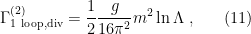
where, for future purposes, we’ve replaced the simple pole in with (this is not an obvious replacement, but follows by comparing the result here with what one would have obtained in the cutoff prescription).

The reason we only identify the beta function with the divergent piece is because, as stated above, we want to identify a function that describes the running of the couplings as we dial the energy scale. Furthermore, we want a description that does not depend on the details of our regularization scheme. With this in mind, observe that there are three kinds of terms in (10). The convergent (constant) terms have no dependence on the cutoff, and therefore won’t tell us anything about the running of the couplings. Terms that diverge as to some positive power , meanwhile, essentially give the relationship between the bare couplings and the renormalized values at a particular scale, but don’t tell us anything about the flow between scales. The log divergence is therefore the only interesting term in this regard: it isn’t associated with any particular scale (said differently, it receives contributions from all scales), and is insensitive to any scheme-dependent behaviour (such as exhibited in the constant terms). Before we proceed, it is worth noting that while dimensional regularization does provide a useful tool for regulating individual loop integrals over the full range , it does not guarantee finiteness of the path integral as in the Wilsonian approach (where the UV regime is simply absent). Additionally, while the Wilsonian cutoff has a physical interpretation as the energy scale, the non-integer status of the dimensions has no such ontic value. Nevertheless, it is of great practical convenience, particularly in gauge theories.

Now, to continue our search for the beta function, let us repeat the above for the 1-loop contribution to the 4-point function,

which occurs at order . The integral in this case is more involved, but can be managed with the use of Feynman’s trick,

which is explained in, e.g., Jim Cline’s Advanced QFT notes. After a fair amount of work, dimensional regularization eventually yields

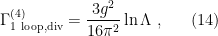
for the singular contribution.

Having regularized the divergences in (11) and (14), we must now renormalize the Lagrangian appropriately. The simplest means of doing so is the minimal subtraction scheme, wherein we only compensate for divergences arising at the one-loop level. The idea is to define a bare Lagrangian

where is the original Lagrangian, and is the Lagrangian consisting of counterterms to compensate for divergences. In the present example of theory,

where the subscript zero denotes that the fields and couplings are bare quantities. These do not depend on , but include the contributions from divergences and are therefore infinite. This is in contrast to the renormalized quantities (without subscript) implicit on the r.h.s. of (15). We shall determine the precise relationship between the bare and renormalized parameters below; it relies on the fact that finite values for the latter are obtained through the introduction of the Lagrangian of counterterms,

where the coefficients , , and , are fixed by our considerations above by observing that, at tree level, yields additional contributions to the vertex functions of the form

Therefore, if we wish to cancel the divergences (11) and (14), we must define

so that, to one-loop level, the total contribution no longer has a divergence as . (In the language of dimensional regularization, we’ve removed the simple pole at ).

Of course, had we gone beyond the minimal subtraction scheme to consider higher loops, additional counterterms would be required (for example, becomes non-trivial at 2-loops). But it turns out that the same basic idea can be performed systematically to all orders in perturbation theory. This is the subject of multiplicative renormalization, which consists in showing that all infinities can be reabsorbed in a finite number of coupling constants (including masses). Finite results are then obtained in the infinite cutoff limit, (equivalently in the dimensional approach), which corresponds to including the full UV regime of the original theory. Theories in which this program can be carried out successfully are called renormalizable. (In fact, renormalizability implies that all counterterms are of the same form as those in the original Lagrangian, which we already assumed in (17)). In contrast, theories requiring an infinite number of counterterms are non-renormalizable—gravity being the most notorious example.

To relate the bare quantities (, , ) to the renormalized quantities (, , ) requires one more piece of information, namely the behaviour of the kinetic term as we change the energy scale. Recalling the Wilsonian approach above, this term is no different than the others in that it receives quantum corrections as we integrate out UV modes. We thus define the field renormalization factor (not to be confused with the partition function ), which depends on such that . (In fact, in the Wilsonian approach, this is sometimes labeled , to reflect the fact that at a new scale , renormalizing the field requires a different factor . But here we only care about the final result; again, the RG is associative). Now, comparing and , we have

At this level, these expressions already describe how the couplings vary, but this is made more concrete in the renormalization group equation (a.k.a. the Callan-Symanzik equation), which we now derive.

First, observe that the field renormalization factor implies that the bare and renormalized -point correlators are related by an overall scaling,

which simply follows from the fact that there are -fields in the correlation function, i.e.,

Since is independent of , it should remain unchanged under RG, hence

And therefore, by the chain rule,

Multiplying through by , we obtain the aforementioned RG equation,

where we have defined

The first of these is the promised beta function, while and are the anomalous dimension of the mass and field, respectively. The name stems from the fact that the renormalized correlation function behaves as if the field scaled with mass dimension rather than ; similarly for . Both of these can be viewed as beta functions for the mass and kinetic terms. The former, after all, is fundamentally no different. Indeed, it is a basic exercise to show that if one treats the mass as an interaction term and sums the resulting Feynman diagrams that contribute to the 2-point function to all orders in , one recovers the usual (massive) propagator.

As stated above, the beta function describes the running of the coupling as we flow from the UV to the IR. Operators that are suppressed as we flow into the IR are called irrelevant. Conversely, operators that becomes increasingly important are called relevant. At the border of these two regimes are operators which are unaffected by the energy scale, which are called marginal. (The terminology can be remembered by asking which operators are relevant, in the colloquial sense, for everyday life (i.e., low-energy physics)). Modulo one significant caveat that we’ll mention shortly, this behaviour can be read-off directly from the Lagrangian. Since the action must be dimensionless, and the measure has mass dimension (and ) the parameters in the Lagrangian must have

However, the perturbative expansion relies on setting, e.g., , which makes no sense if is dimensionful. More generally, for a given coupling with , implies that the correct dimensionless parameter is , and thus controls an interaction that becomes increasingly important at low energies . In this case the hypothetical term is relevant. Conversely, implies that we perform an expansion in , in which case the interaction becomes less and less important as becomes small; hence, irrelevant. The marginal case is , in which case we really can expand in , since it’s already dimensionless.

The aforementioned caveat is that quantum corrections can modify the RG behaviour of the coupling. In the example above, the classical mass dimension of the field in theory is modified by the anomalous dimension . In particular, one must watch out for marginal operators that become either marginally relevant or marginally irrelevant under RG. Such operators actually play an important role in phenomenology. More generally, the fact that operators can mix under RG flow is important in, for example, the possible emergence of gauge fields.

The existence of an infinite-dimensional space of theories whose coordinates is the set of all possible couplings in the effective action implies the existence of an infinite number of irrelevant operators. In contrast, since each additional field or derivative increases the dimension of an operator, there are only finitely many relevant operators (and typically very few). We define the critical surface to be the infinite-dimensional space in the UV where all relevant operators vanish (which has finite codimension, for the reason just stated). As we flow to the IR — which we might accomplish by perturbing away from the critical surface by the introduction of some relevant operator(s) — we follow a trajectory through the space of theories until we reach a critical or fixed point, where all beta functions vanish. If the beta function has a zero at , and is positive for , then as . In this case, is a UV fixed point. Alternatively, if for , then as ; since we dialed the energy in the same direction, it’s still a UV fixed point, but the vanishing of the coupling implies that the theory becomes asymptotically free, a feature that characterizes certain non-abelian gauge theories, notably QCD. An IR fixed point, in obvious contrast, is obtained from a similar analysis with (though asymptotic freedom uniquely refers to the UV case).

Another case that deserves mention is the possibility that the beta function diverges at some finite . This is an obvious pathology, since it implies that the coupling constant — i.e., the interaction strength — becomes infinite. But in fact, this is precisely what happens in our beloved theory, and is a common feature of theories which are not asymptotically free, such as QED. One possible solution to this is that the fully renormalized coupling actually goes to zero as we take the cutoff scale to infinity. The proposed mechanism by which this quantum triviality comes about is via vacuum fluctuations (essentially, corrections from the self-energy of the field), which completely screen the interaction in the absence of a cutoff. (This is sometimes referred to as charge screening, in analogy with electrodynamics). The alternative is to suppose that the perturbative expansion simply breaks down at strong coupling, since the pathology appears at one- or two-loop level, in which case non-perturbative methods must be used to address the issue, such as in lattice gauge theory. We don’t normally concern ourselves with triviality in theory, because the energy scale at which it occurs is inaccessibly high. However, field theories involving only a scalar Higgs boson in four dimensions also suffer from quantum triviality, but at a scale that may be accessible to the LHC; the possible inconsistency of such theories is an open area of research.

There is of course a great deal more to be said about the RG; see for example Skinner’s explanation for how it vastly simplifies the Feynman diagram expansion, or Polchinski’s interpretation of RG as a form of heat flow. There’s also the interesting fact that the RG flow entails a shift in the vacuum energy (Skinner, page 39), which suggests both complications for renormalization in curved spacetime as well as a tantalizing hint towards the emergence of the radial direction in AdS/CFT—namely, holography as RG flow, a fascinating research direction in its own right.