
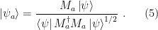
In an earlier post, we sketched the basic mathematical description of quantum mechanics, culminating in the general description of quantum states as (reduced) density matrices. We also claimed that generic measurements are not orthogonal projections, and evolution is not unitary. We shall here expand upon the aforementioned infrastructure to explain these statements, resolving some un-answered questions in the process. We shall again draw from Preskill’s Quantum Information and Computation course notes, as well as a lecture given by Mario Flory on POVMs and superoperators.
The naïve picture is that, as a consequence of Schmidt decomposition, one can write the density matrix for a mixed state as an ensemble of orthogonal pure states, the eigenvalues of which are interpreted as the probability of their occurring. When we measure the system, we project onto one of these eigenstates, hence the notion of measurements as orthogonal projections. And indeed this works fine for isolated systems; but as explained previously, this is an idealization. The problem that demands a more generalized notion of measurement is that an orthogonal measurement in a tensor product 

Let us first make the notion of orthogonal projections a bit more precise, following von Neumann’s treatment thereof. To perform a measurement of an observable 


where in the second equality we’ve expanded 
![{\left[M,H_0\right]=0}](https://s0.wp.com/latex.php?latex=%7B%5Cleft%5BM%2CH_0%5Cright%5D%3D0%7D&bg=ffffff&fg=000000&s=0&c=20201002)

Since 


Now the position of the pointer is correlated with the value of the observable 


Of course, in principle the measurement process could project out some superposition of eigenstates, rather than a single position eigenstate as in the above example. Indeed, if we can couple any observable to a pointer, then we can perform any orthogonal projection in Hilbert space. Thus to formulate the above more generally, consider a set of projection operators 


with probability

as usual.
Thus far we have been referring to measurements on a single isolated Hilbert space, for which PVMs suffice. But in practice we only ever deal with subsystems, for which our concept of measurement must be suitably extended. As we shall see, the relevant entities for the job are positive operator valued measures, or POVMs. The key difference between a POVM and a PVM is that the latter are a subset of the former for which the eigenstates are orthogonal by construction.
Mathematically, a POVM is a measure (basically, a partition of unity) whose values are non-negative self-adjoint operators on Hilbert space. That is, denoting the set of operators that comprise the POVM by 


Given the positivity of the operators 

Note that this expression is precisely the same as that given for PVMs above; in other words, 


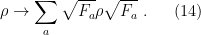
To elaborate on this slightly further, let us take the familiar example of a tensor product space 


We may obtain an explicit expression for
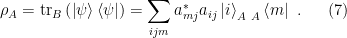
Since 


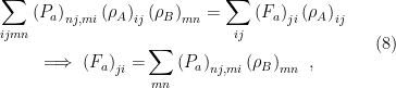
where 


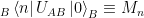
As one might have expected given that POVMs act on subspaces, a POVM can be lifted to a PVM by expanding the Hilbert space of the former and performing the latter in the resulting superspace. This is the content of Neimark’s (sometimes transliterated from the Cyrillic “Ðаймарк” as “Neumark”) theorem. Note that the converse also holds: any PVM on a Hilbert space reduces to a POVM on any subspace thereof. This means that one can realize a POVM as a PVM on an enlarged Hilbert space, which allows one to obtain the correct measurement probabilities (by which we mean, the relative weights in the ensemble; see below) by performing orthogonal projections. Conversely, an orthogonal measurement of a bipartite system
In addition to the crucial role they play in measurement, POVMs are useful for formulating a suitable generalization of evolution that applies to subsystems. By way of example, suppose the initial state in 


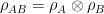
whereupon the density matrix of subsystem

where 


We may thus expression 
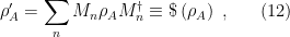
where 


The mapping 


In addition to these three necessary properties, it is also customary to assume that
Unitary evolution, for an isolated system, is described by the Schrödinger equation. The analagous equation for general evolution by superoperators is called the Master equation. Preskill elaborates on this in some detail in section 3.5, but we will restrain ourselves from getting involved in such details here. Instead, we merely observe that unitary evolution can be thought of as the special case in which the operator sum contains only a single term. Under unitary evolution, pure states can only evolve to pure states:

and similarly mixed states remain mixed. But superoperators allow the evolution of pure states to mixed states. This is called decoherence. It is the process by which initially pure states become entangled, and consequently, it plays a fundamental role in both the mathematics of quantum mechanics and the (philosophical) interpretation thereof.
To connect back to our earlier example, suppose we perform a POVM on
By Neimark’s theorem, the POVM

In other words, the bipartite system undergoes a unitary transformation that entangles

We could thus describe the measurement by a PVM on 

where the second equality follows from comparison with (6). Normalizing the final state accordingly, we may write (14) as

We mentioned previously that for POVMs, repeated measurements will not necessarily yield the same result. Now we see why: the result of such a general measurement (that is, on a subsystem) is given an ensemble of pure states, and thus we require a description in terms of a density matrix rather than as a single (orthogonal) eigenstate.
This is also the description we would use if we knew only that a measurement had been performed, but were ignorant of the results. For example, suppose we perform a measurement by probing the system with a single particle (say, a photon from a laser). Immediately after the interaction with the probe, but before the interaction with the classical detector that records it, the system is in an entangled state. We would thus describe the process as evolution by a superoperator that produces a density matrix/ensemble as above. In other words, the system has slightly decohered: if the initial state were pure, some of the coherence has been lost upon evolution to a mixed state. The subsequent interaction with the (classical) detector that we colloquially think of as “measurement” is simply the same process of decoherence on a hugely expanded scale: the (now mixed) state becomes entangled with the trillions of particles that comprise the detector, decohering essentially instantaneously to a classical state. All the uniquely quantum information of the system has now been lost.
This is what is referred to as “collapse of the wavefunction” in the Copenhagen interpretation. The reason for the invalidity of this interpretation is that it posits a projection onto a single eigenstate as a result of observation (by which we simply mean, interaction with the measurement apparatus; anthropocentric language aside, consciousness is emphatically not involved in any fundamental way). But as we’ve seen above, a proper description of measurement is that of entanglement with the environment under evolution via superoperators. The measurement process proceeds by POVMs, not PVMs, on the (sub)system under study. And while at the end of the day one does arrive at an eigenstate in the expanded Hilbert space (that includes the measurement apparatus/detector/observer/etc), this is a consequence of decohering to a classical state, rather than directly projecting to it. Decoherence can thus be thought of as giving the appearance of wavefunction collapse; but as evidenced by the countless reams of confused literature on quantum foundations and related areas, it is most dangerous to indulge in such simplifications so blithely. (We note in passing that the “wavefunction of the universe” never decoheres, since evolution in an isolated system is unitary).
Another important fact that no doubt contributes to the collapse confusion is that decoherence is irreversible. Consider composing two superoperators to form a third: if 


Several open questions remain. Perhaps chief among them is our failure to fully resolve the “disconcerting dualism” between deterministic evolution and probabilistic measurement. Insofar as probability is a statement of our ignorance and thus fundamentally epistemic, any formulation of quantum mechanics that relies thereupon is doomed to suffer the same characterization, for what does it mean to say that nature is fundamentally probabilistic? We may ask whether the associated lack of predictivity in quantum mechanics stems from the fact that there does not exist a state which is an eigenstate of all observables. One also wonders whether it is possible to formulate a consistent theory with non-linearly evolving superoperators, and what the interpretation thereof would be vis-à-vis probabilistic ensembles (that is, to what extent we can free ourselves from probability if we distance ourselves from the linearity it imposes). Zurek’s work on decoherence contains some clarifying insight into this issue, but that’s a subject for another post.
It is tempting to speculate that the issue of how to properly describe measurement and evolution lies at the heart of the black hole information paradox, wherein a black hole formed from the collapse of an initially pure state appears to evolve to a mixed state, in violation of the supposedly unitary S-matrix. Indeed, for various reasons, this picture is almost certainly too naïve. In particular, evolution is not unitary, but it remains to be shown precisely how a more ontologically accurate rendition of the problem would solve it.
