Action integrals and partition functions

There’s a marvelous — and by now quite well-known — paper (paywalled) by Gibbons and Hawking, in which they compute the entropy of black holes from what is essentially a purely geometrical argument. This relies on the fact that the partition function has an expression in terms of both a path integral and a statistical ensemble. The former allows one to solve for the gravitational action, and the latter endows this with a standard thermodynamic interpretation.

In the path integral formulation, one expresses the generating functional of correlation functions as

$\displaystyle Z=\int\mathcal{D}g\mathcal{D}\phi e^{iI[\phi]} \ \ \ \ \ (1)$

where ${I}$ is the action functional of the fields ${\phi}$ (to avoid confusion, we’ll use ${I}$ for action in order to reserve ${S}$ for entropy). Gibbons and Hawking begin by pointing out that, in the case of black holes, the presence of spacetime singularities prevents one from evaluating the action. However, one can side-step this difficulty by Wick rotating to Euclidean signature, whereupon the geometry pinches off smoothly at the event horizon, thus providing one with a non-singular, compact manifold on which to evaluate the action. Let’s see how this works.

In ${3+1}$ dimensions, the gravitational action is

$\displaystyle I=\frac{1}{16\pi}\int\mathrm{d}^4x\sqrt{-g}R~. \ \ \ \ \ (2)$

However, the Ricci scalar ${R}$ contains second-order derivatives with respect to the metric:

$\displaystyle R=2g^{\mu\nu}\left(\Gamma^\rho_{\mu\left[\nu,\rho\right]}+\Gamma^\sigma_{\mu\left[\nu\right.}\Gamma^\rho_{\left.\rho\right]\sigma}\right)~,\;\;\; \Gamma_{\rho\mu\nu}=\frac{1}{2}\left( g_{\rho\mu,\nu}+g_{\rho\nu,\mu}-g_{\mu\nu,\rho}\right)~, \ \ \ \ \ (3)$

which implies that the action suffers from an Ostrogradski instability, and is thus unsuitable for the path integral approach. One can remedy this via partial integration, but that requires that we properly account for boundary terms. A more complete expression for the above action is therefore

$\displaystyle I=\frac{1}{16\pi}\int_M\mathrm{d}^4x\sqrt{-g}R+\frac{1}{8\pi}\int_{\partial M}\mathrm{d}^3x\sqrt{-h}K~. \ \ \ \ \ (4)$

where ${M}$ is the spacetime manifold with boundary ${\partial M}$ . The second term is known as the Gibbons-Hawking-York boundary term, where ${h_{\mu\nu}}$ is the induced metric on ${\partial M}$ and ${K}$ is the trace of the second fundamental form. (Recall that the first fundamental form is the inner product induced on the tangent space of a surface ${\mathcal{S}}$ in ${\mathbb{R}^3}$ by the dot product on the latter. The second fundamental form is a quadratic form on the tangent plane of ${\mathcal{S}}$ . Collectively these allow the definition of extrinsic curvature invariants.)

Two quick technical notes are in order. First, in the above expression, we have the freedom to add a constant ${C}$ to the boundary term that depends only on the induced metric ${h_{\mu\nu}}$ . However, since this is independent of ${g_{\mu\nu}}$ , it can be absorbed in the normalization of the measure on the space of all metrics. For convenience, we choose this constant so that in the asymptotically flat spacetimes with which we’re concerned, ${I=0}$ for the flat-space metric ${\eta_{\mu\nu}}$ . Therefore ${K}$ should be understood to mean the difference in the trace of the second fundamental form of ${\partial M}$ in the metrics ${g_{\mu\nu}}$ and ${\eta_{\mu\nu}}$ .

Secondly, the second fundamental form is a ${(0,2)}$ -tensor, and hence does not have a trace in the strictest sense (since the trace should not be coordinate dependent, while ${\mathrm{tr}K=\sum_i K_{ii}}$ clearly is). Thus when one speaks of the trace of ${K}$ in the metric ${g_{\mu\nu}}$ , one means the trace over or with respect to the metric, i.e. ${\mathrm{tr}_gK\equiv\mathrm{tr}\left( g^{-1}K\right)=\sum_{ij}g^{ij}K_{ij}=K^i_{~i}}$ (this last is a ${(1,1)}$ -tensor, and is therefore coordinate independent, as desired).

We will now proceed to evaluate the above action for the Schwarzschild black hole, given by the intimately familar metric

$\displaystyle \mathrm{d} s^2=-f(r)\mathrm{d} t^2+\frac{1}{f(r)}\mathrm{d} r^2+r^2\mathrm{d}\Omega^2~,\;\;\;f(r)=1-\frac{r_s}{r}~, \ \ \ \ \ (5)$

where the event horizon ${r_s=2M}$ . We shall henceforth suppress the 2-sphere ${\mathrm{d}\Omega^2}$ , as it plays no role in the following. As is well-known, the Schwarzschild metric has singularities at ${r=0}$ and ${r=r_s}$ , but the latter is merely a coordinate singularity and can by removed by transforming to (among other things) Kruskal coordinates:

$\displaystyle \mathrm{d} s^2=\frac{4r_s^2}{r^3}e^{-r/r_s}\left(-\mathrm{d} T^2+\mathrm{d} X^2\right) \ \ \ \ \ (6)$

where

$\displaystyle T^2-X^2=f(r)e^{r/r_s}~,\;\;\;\frac{X+T}{X-T}=e^{t/r_s}~. \ \ \ \ \ (7)$

These coordinates are regular throughout the whole spacetime; in particular, although the signs of ${T}$ and ${X}$ change as one crosses to the interior, there’s nothing pathological at the horizon itself. Additionally, note that the curvature singularity ${r=0}$ has been mapped to the hyperbola ${T^2-X^2=1}$ .

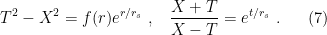
Now comes the magic. We Wick rotate to Euclidean signature by defining a new coordinate ${\xi=iT}$ . Aside from the obvious sign change in the metric, this changes the definition of ${r}$ to

$\displaystyle \xi^2+X^2=\left(\frac{r}{r_s}-1\right) e^{r/r_s}, \ \ \ \ \ (8)$

and thus if we restrict to ${\xi,X\in\mathbb{R}}$ , we must have ${r\ge r_s}$ . In other words, the Euclidean black hole has no interior; the geometry stops at the horizon!

There’s a cute way to visualize this geometry rather easily. Go back to the Schwarzschild metric above and zoom in near the horizon:

$\displaystyle f(r)\big|_{r_s}=f(r_s)+(r-r_s)\partial_rf(r)\big|_{r_s}+O(r^2)=\frac{r-r_s}{r_s} \ \ \ \ \ (9)$

where in the last step we’ve dropped higher-order terms. It will then be convenient to rewrite the metric in terms of the proper distance ${\rho}$ near the horizon, which is found as follows:

$\displaystyle \frac{\mathrm{d} r^2}{f(r)}=\mathrm{d}\rho^2\implies\frac{\mathrm{d} r}{\sqrt{\frac{r}{r_s}-1}}=\mathrm{d}\rho\implies \frac{r}{r_s}-1=\frac{\rho^2}{4r_s^2}~. \ \ \ \ \ (10)$

Thus, after Wick rotating to ${\tau=it}$ , we have

$\displaystyle \mathrm{d} s^2=\mathrm{d}\rho^2+\frac{\rho^2}{4r_s^2}\mathrm{d}\tau^2~. \ \ \ \ \ (11)$

But this is merely the line element in polar coordinates! And in polar coordinates, we must identify ${\frac{\tau}{2r_s}\sim\frac{\tau}{2r_s}+2\pi}$ to avoid a conical deficit. This is one of many ways to see that Wick rotation leads to periodicity in imaginary time.

The following is a sketch of the resulting geometry. The radial coordinate increases towards the right, while the periodic ${\tau}$ coordinate forms the circumference of the “cigar”. Each point on the surface is an ${S^2}$ , from the suppressed 2-sphere ${\mathrm{d}\Omega}$ . Note that, as explained above, the geometry pinches off smoothly at the horizon: the end-point at the left is at ${r_s}$ .

EuclideanBH

As an aside, the Euclidean vacuum is known as the Hartle-Hawking vacuum state, which is subtly yet crucially different than the (more physically relevant) Unruh vacuum. This is an important point when one wishes to discuss thermodynamic effects like Hawking radiation, but the distinction is a subject for another post.

This is the crucial enabling factor that allows one to compute the action: the Euclidean section is non-singular, and hence ${S}$ can be evaluated on a region ${M}$ bounded by some surface ${r=r_0>2M}$ , whose boundary ${\partial M}$ has compact topology ${S^1\times S^2}$ (periodic time cross the suppressed ${\mathrm{d}\Omega^2}$ ).

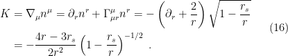
Since the Ricci scalar vanishes in the Schwarzschild metric, the action is entirely determined by the Gibbons-Hawking-York boundary term. Rewriting the integration measure as an area element ${\mathrm{d}\Sigma}$ , this becomes

$\displaystyle I=\frac{1}{8\pi}\int\!K\mathrm{d}\Sigma =\frac{1}{8\pi}\int \nabla_\mu n^\mu\mathrm{d}\Sigma~, \ \ \ \ \ (12)$

where the appropriate normal vector ${n^\mu}$ is found from the bulk metric ${g_{\mu\nu}}$ by simply normalizing with respect to the ${\mathrm{d} r^2}$ component ${f(r)^{-1}}$ :

$\displaystyle n^\mu=-\frac{\delta^{\mu r}}{\sqrt{f(r)^{-1}}}\implies n^r=-\sqrt{1-\frac{r_s}{r}}~. \ \ \ \ \ (13)$

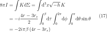
This is an integral over the boundary ${S^1\!\times\!S^2}$ at ${r=r_0}$ , with induced metric

$\displaystyle \mathrm{d} s^2=\left(1-\frac{r_s}{r}\right)\mathrm{d}\tau^2+r^2\mathrm{d}\Omega^2\;\;\; \implies\;\;\; \sqrt{-h}=ir^2\sin\theta\sqrt{1-\frac{r_s}{r}}~, \ \ \ \ \ (14)$

Now, there are two ways to evaluate this integral. The most straightforward option is to directly compute ${K=\nabla_\mu n^\mu}$ . Since the covariant derivative generally involves non-trivial Christoffel symbols, I’m going to call this the brute-force method. Of course, these are well-known for the Schwarzschild metric, so in this case we may simply write down the relevant components:

$\displaystyle \Gamma_{tr}^t=-\Gamma_{rr}^r=\frac{r_s}{2r^2}\left(1-\frac{r_s}{r}\right)^{-1}~,\qquad \Gamma_{\theta r}^\theta=\Gamma_{\phi r}^\phi=\frac{1}{r}~. \ \ \ \ \ (15)$

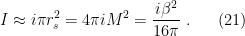
We therefore have

$\displaystyle \begin{aligned} K&=\nabla_\mu n^\mu=\partial_r n^r+\Gamma_{\mu r}^\mu n^r =-\left(\partial_r+\frac{2}{r}\right)\sqrt{1-\frac{r_s}{r}}\\ &=-\frac{4r-3r_s}{2r^2}\left(1-\frac{r_s}{r}\right)^{-1/2}~. \end{aligned} \ \ \ \ \ (16)$

Substituting (14) and (16) into the integral expression (12), we have

$\displaystyle \begin{aligned} 8\pi I&=\int\!K\mathrm{d}\Sigma =\int\!\mathrm{d}^3x\sqrt{-h}\,K\\ &=-i\frac{4r-3r_s}{2}\int_0^\beta\!\mathrm{d}\tau\int_0^{2\pi}\!\mathrm{d}\phi\int_0^\pi\!\mathrm{d}\theta\sin\theta\\ &=-2i\pi\beta\left(4r-3r_s\right) \end{aligned} \ \ \ \ \ (17)$

Alternatively, a more elgant method that avoids the need to compute the curvature (read: Christoffel symbols) is to integrate by parts. After recognizing the directional derivative ${n^\mu\nabla_\mu=\partial_n}$ , and using the fact that ${n^\mu\cdot\mathrm{d}\Sigma=0}$ by definition, one obtains

$\displaystyle 8\pi I=\partial_n\int\mathrm{d}\Sigma =-\sqrt{1-\frac{r_s}{r}}\,\partial_r\left(4\pi\beta ir^2\sqrt{1-\frac{r_s}{r}}\right) =-2i\pi\beta\left(4r-3r_s\right)~. \ \ \ \ \ (18)$

We’re not quite done though: we want to ensure that our geometrical result includes only the contribution of the black hole geometry, not any flat space contribution, so we need to renormalize by subtracting the latter. To do so, we’ll push the surface ${r_0}$ to infinity, where any deviation from Minkowski space is due to the ${U(1)}$ symmetry (analagous to the global effect of a conical deficit). We alluded to this above, when we used ${K}$ as a shorthand notation for ${\mathrm{tr}_g(K)-\mathrm{tr}_\eta(K)}$ . We just calculated the first term; now let’s do the second.

We have the same induced metric, but embedding this boundary geometry in flat space means that the covariant derivative reduces to the divergence of the normal vector, and we can use the original form of the integral expression directly. The unit normal is ${n^r=-1}$ , so ${K=r^{-2}\partial_r\left( r^2(-1)\right)=-2/r~}$ . Plugging these components into the action, and evaulating with the same limits as above, we have the flat-space contribution ${I_0}$ :

$\displaystyle (8\pi)I_0=-8i\pi\beta r\sqrt{1-\frac{r_s}{r}}~. \ \ \ \ \ (19)$

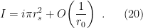
Finally, taking the difference of (18) and (19), and Taylor expanding around ${r_0\rightarrow\infty}$ (keep in mind that ${r}$ in the above expressions is really ${r_0}$ , the boundary of the integration region on the cigar), one finds

$\displaystyle I=i\pi r_s^2+O\!\left(\frac{1}{r_0}\right)~. \ \ \ \ \ (20)$

Using the fact that ${\beta=8\pi M}$ and ${r_s=2M}$ , we thus have the leading-order contribution

$\displaystyle I\approx i\pi r_s^2= 4\pi i M^2=\frac{i\beta^2}{16\pi}~. \ \ \ \ \ (21)$

It’s essential to note that we’ve computed the dominant saddle point here. The path integral is dominated by the metric ${g}$ and fields ${\phi}$ that satisfy the classical field equations, since these extremize the action by definition. We then expand around these values such that ${g=g_0+\tilde g}$ , ${\phi=\phi_0+\tilde\phi}$ , and

$\displaystyle I[g,\phi]=I[g_0,\phi_0]+\ldots \ \ \ \ \ (22)$

where the ellipsis denotes terms that are quadratic and higher in fluctuations about the background values. The leading-order contribution to the partition function is therefore

$\displaystyle Z=e^{iI[g_0,\phi_0]}\implies \ln Z=iI[g_0,\phi_0]=-\frac{\beta^2}{16\pi} \ \ \ \ \ (23)$

where we’ve expressed the result in terms of ${\beta}$ to fascillitate subsequent manipulations.

Gibbons and Hawking go on to compute the action for more general black holes as well, including the Reissner-Nordström solution, but we’re more concerned with the underlying physics than the mathematical details here, so let’s jump ahead to the second part of the paper, where we’ll see just what wonders these seemingly innocuous manipulations have wrought.

In fact, the answer is forshadowed already in the expression above: ${\pi r_s^2}$ is precisely a fourth the area of the horizon. But so far this is an expression for an action, not an entropy. To make the connection betwixt them, we’ll need some thermodynamics.

First, recall that the total energy of a thermodynamic system in the canonical ensemble is found by summing over the microstates (that is, energy eigenstates ${E_i}$ ) weighted by their probabilities ${P_i}$ :

$\displaystyle \left<E\right>=\sum_iE_iP_i=\frac{1}{Z}\sum_iE_ie^{-\beta E_i}=-\frac{1}{Z}\partial_\beta Z=-\partial_\beta\ln Z~. \ \ \ \ \ (24)$

We shall use this to obtain a particular expression for the entropy,

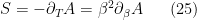
$\displaystyle S=-\partial_TA=\beta^2\partial_\beta A \ \ \ \ \ (25)$

where in the second equality we’ve simply rewritten the thermal derivative via ${T=\beta^{-1}}$ . ${A}$ is the Helmholz free energy,

$\displaystyle A=\left<E\right>-TS=-\beta^{-1}\ln Z~. \ \ \ \ \ (26)$

The derivation is quite simple:

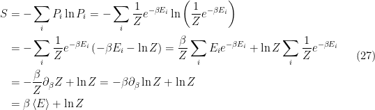
$\displaystyle \begin{aligned} S&=-\sum_i P_i\ln P_i=-\sum_i\frac{1}{Z}e^{-\beta E_i}\ln\left(\frac{1}{Z}e^{-\beta E_i}\right)\\ &=-\sum_i\frac{1}{Z}e^{-\beta E_i}\left(-\beta E_i-\ln Z\right) =\frac{\beta}{Z}\sum_iE_ie^{-\beta E_i}+\ln Z\sum_i\frac{1}{Z}e^{-\beta E_i}\\ &=-\frac{\beta}{Z}\partial_\beta Z+\ln Z =-\beta\partial_\beta \ln Z+\ln Z\\ &=\beta\left<E\right>+\ln Z \end{aligned} \ \ \ \ \ (27)$

where in going to the third line we’ve used the fact that ${\sum_i P_i=1}$ . Now, from the definition of the Helmholtz free energy,

$\displaystyle \begin{aligned} A&=-T\ln Z\implies\\ \partial_TA&=-\ln Z-T\partial_T\ln Z\implies\\ -\beta^2\partial_\beta A&=-\ln Z+\beta\partial_\beta\ln Z\implies\\ \beta^2\partial_\beta A&=\ln Z+\beta\left<E\right> \end{aligned} \ \ \ \ \ (28)$

Thus

$\displaystyle S=\beta\left<E\right>+\ln Z=\beta^2\partial_\beta A \ \ \ \ \ (29)$

as desired.

Now our famous result is more-or-less immediate. From our above expression for the Lorentzian action, we have the dominant contribution to the path integral,

$\displaystyle \ln Z=-\frac{\beta^2}{16\pi}~, \ \ \ \ \ (30)$

and therefore the free energy is

$\displaystyle A=-\beta^{-1}\ln Z=\frac{\beta}{16\pi}~. \ \ \ \ \ (31)$

Substituting this into above expression for entropy, one finds

$\displaystyle S=\frac{\beta^2}{16\pi}=\pi r_s^2=\frac{\mathrm{Area}}{4} \ \ \ \ \ (32)$

voilà!

Several comments are in order. First, one might be concerned that in the course of the saddle point approximation, we missed out on important corrections. This is not the case: as explained in the paper, the higher order terms merely correspond to contributions from thermal gravitions and matter quanta (which technically requires the Gibbs, rather than Helmholtz, free energy to properly take into account the non-zero chemical potential). But we’re only interested in the “background” contribution from the horizon itself; as alluded in the introductory paragraph, this is a purely geometrical effect, which is entirely represented in the leading order term.

Though the path integral is in some sense an inherently quantum mechanical object, it is remarkable that we were able to obtain this result by otherwise appealing solely to classical geometry and thermodynamics. In particular, the fixed point of the ${U(1)}$ symmetry ( ${\tau\sim\tau+\beta}$ ) featured crucially in the analysis. An extension of this method, where the fixed points form a conical deficit, can be shown to yield the same result. Indeed, the same feature lies at the heart of the recent proof of the Ryu-Takayanagi proposal by Lewkowycz and Maldacena, where the above geometrical computation of horizon entropy is extended to holography. Given the inextensibility (so far) of most of the other myriad ways of computing black hole entropy (e.g. Hawking pairs, string microstates, Noether charge) to arbitrary spacetime horizons, this further suggests a deep connection between entropy and geometry; one which we are only beginning to unravel.

6 Responses to Action integrals and partition functions

Anish Bhattacharya says:

July 7, 2020 at 8:05 pm

One doubt: How do we know that Wick rotating to Euclidean signature gives us the correct answer? I understand that it helps us evaluate the action integral in a neat fashion, and I don’t know if this is a stupid question, but what if we missed something because of that? Since physically, it’s still a Schwarzschild metric in Lorentz signature.

LikeLike

Pingback: Islands behind the horizon | Ro's blog
lucab1992 says:

November 10, 2021 at 2:11 pm

Hi Ro, very nice post!
I just wanted to mention one small typo in the first line: it should be “Gibbons” and not “Giddings” :-p

LikeLike

- rojefferson says:
  
  November 26, 2021 at 1:28 pm
  
  Whoops, thanks Luca; fixed!
  
  LikeLike
  
minjukum says:

November 2, 2022 at 5:44 am

Hi Ro, thanks a lot for the post.
Could you explain why in (13) the unit normal has the minus sign?

LikeLike

- rojefferson says:
  
  November 8, 2022 at 12:07 pm
  
  The sign of the unit normal vector denotes the orientation, namely inwards (negative) or outwards (positive).
  
  What we’re ultimately after here is the extrinsic curvature: intuitively, if ${T(s)}$ is some tangent vector to the hypersurface at point ${s}$ , then the derivative of ${T}$ with respect to ${T(s)}$ tells us how much the surface curves as we move along it. Mathematically, this derivative is a vector normal to the surface, whose length gives the curvature. In particular, one can see pictorially that the normal vector thus defined will point towards the center of curvature, which in this case is the tip of the cigar—i.e., inwards, hence the negative sign.
  
  LikeLike