As part of my ongoing love affair with black holes, I’ve been digging more deeply into what it means for them to have entropy, which of course necessitates investigating how this is assigned in the first place. This is a notoriously confusing issue — indeed, one which lies at the very heart of the firewall paradox — which is further complicated by the fact that there are a priori three distinct physical entropies at play: thermodynamic, entanglement, and gravitational. (Incidentally, lest my previous post on entropy cause confusion, let me stress that said post dealt only with the relation between thermodynamic and information-theoretic a.k.a. Shannon entropy, at a purely classical level: neither entanglement nor gravity played any role there. I also didn’t include the Shannon entropy in the list above, because — as explained in the aforementioned post — this isn’t an objective/physical entropy in the sense of the other three; more on this below.)

My research led me to a review on black hole entanglement entropy by Solodukhin [1], which is primarily concerned with the use of the conical singularity method (read: replica trick) to isolate the divergences that arise whenever one attempts to compute entanglement entropy in quantum field theory. The structure of these divergences turns out to provide physical insight into the nature of this entropy, and sheds some light on the relation to thermodynamic/gravitational entropy as well, so these sorts of calculations are well-worth understanding in detail.

While I’ve written about the replica trick at a rather abstract level before, for present purposes we must be substantially more concrete. To that end, the main technical objective of this post is to elucidate one of the central tools employed by these computations, known as the heat kernel method. This is a rather powerful method with applications scattered throughout theoretical physics, notably the calculation of 1-loop divergences and the study of anomalies. Our exposition will mostly follow the excellent pedagogical review by Vassilevich [2]. Before diving into the details however, let’s first review the replica trick à la [1], in order to see how the heat kernel arises in the present context.

Consider some quantum field in -dimensional Euclidean spacetime, where with . The Euclidean time is related to Minkowski time via the usual Wick rotation, and we have singled-out one of the transverse coordinates for reasons which will shortly become apparent. For simplicity, let us consider the wavefunction for the vacuum state, which we prepare by performing the path integral over the lower () half of Euclidean spacetime with the boundary condition :

where we have used to denote the Euclidean action for the matter field, so as to reserve for the entropy.

Now, since we’re interested in computing the entanglement entropy of a subregion, let us divide the surface into two halves, and , by defining a codimension-2 surface by the condition , . Correspondingly, let us denote the boundary data

The reduced density matrix that describes the subregion of the vacuum state is then obtained by tracing over the complementary set of boundary fields . In the Euclidean path integral, this corresponds to integrating out over the entire spacetime, but with a cut from negative infinity to along the surface (i.e., along ). We must therefore impose boundary conditions for the remaining field as this cut is approached from above () and below (). Hence:

Formally, this object simply says that the transition elements are computed by performing the path integral with the specified boundary conditions along the cut.

Unfortunately, explicitly computing the von Neumann entropy is an impossible task for all but the very simplest systems. Enter the replica trick. The basic idea is to consider the -fold cover of the above geometry, introduce a conical deficit at the boundary of the cut , and then differentiate with respect to the deficit angle, whereupon the von Neumann entropy is recovered in the appropriate limit. To see this in detail, it is convenient to represent the subspace in polar coordinates , where and , such that the cut corresponds to for . In constructing the -sheeted cover, we glue sheets along the cut such that the fields are smoothly continued from to . The resulting space is technically a cone, denoted , with angular deficit at , on which the partition function for the fields is given by

where is the power of the density matrix (3). At this point in our previous treatment of the replica trick, we introduced the Rényi entropy

which one can think of as the entropy carried by the copies of the chosen subregion, and showed that the von Neumann entropy is recovered in the limit . Equivalently, we may express the von Neumann entropy directly as

Explicitly:

where in the last step we took the path integral to be appropriately normalized such that , whereupon the second term vanishes. Et voilà! As I understand it, the aforementioned “conical singularity method” is essentially an abstraction of the replica trick to spacetimes with conical singularities. Hence, re-purposing our notation, consider the effective action for fields on a Euclidean spacetime with a conical singularity at . The cone is defined, in polar coordinates, by making periodic with period , and taking the limit in which the deficit . The entanglement entropy for fields on this background is then

As a technical aside: in both these cases, there is of course the subtlety of analytically continuing the parameter resp. to non-integer values. We’ve discussed this issue before in the context of holography, where one surmounts this by instead performing the continuation in the bulk. We shall not digress upon this here, except to note that the construction relies on an abelian (rotational) symmetry , where is an arbitrary constant. This is actually an important constraint to bear in mind when attempting to infer general physical lessons from our results, but we’ll address this caveat later. Suffice to say that given this assumption, the analytical continuation can be uniquely performed without obstruction; see in particular section 2.7 of [1] for details.

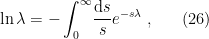
We have thus obtained, in (8), an expression for the entanglement entropy in terms of the effective action in the presence of a conical singularity. And while this is all well and pretty, in order for this expression to be of any practical use, we require a means of explicitly computing . It is at this point that the heat kernel enters the game. The idea is to represent the Green function — or rather, the (connected) two-point correlator — as an integral over an auxiliary “proper time” of a kernel satisfying the heat equation. This enables one to express the effective action as

where is the (trace of the) heat kernel for the Laplacian operator . We’ll now spend some time unpacking this statement, which first requires that we review some basic facts about Green functions, propagators, and all that.

Consider a linear differential operator acting on distributions with support on . If admits a right inverse, then the latter defines the Green function as the solution to the inhomogeneous differential equation

where represent vectors in . We may also define the kernel of as the solution to the homogeneous differential equation

The Green function is especially useful for solving linear differential equations of the form

To see this, simply multiply both sides of (10) by and integrate w.r.t ; by virtue of the delta function (and the fact that is independent of ), one identifies

The particular boundary conditions we impose on then determine the precise form of (e.g., retarded vs. advanced Green functions in QFT).

As nicely explained in this Stack Exchange answer, the precise relation to propagators is ambiguous, because physicists use this term to mean either the Green function or the kernel, depending on context. For example, the Feynman propagator for a scalar field is a Green function for the Klein-Gordon operator, since it satisfies the equation

In contrast, the corresponding Wightman functions

are kernels for this operator, since they satisfy

The reader is warmly referred to section 2.7 of Birrell & Davies classic textbook [3] for a more thorough explanation of Green functions in this context (see also part 1 of my QFT in curved space sequence).

In the present case, we shall be concerned with the heat kernel

where is some Laplacian operator, by which we mean that it admits a local expression of the form

for some matrix-valued functions . In the second equality, we’ve written the operator in the so-called canonical form for a Laplacian operator on a vector bundle, where is an endomorphism on the bundle over the manifold, and the covariant derivative includes both the familiar Riemann part as well as the contribution from the gauge (bundle) part; the field strength for the latter will be denoted . Fibre bundles won’t be terribly important for our purposes, but we’ll need some of this notation later; see section 2.1 of [2] for details.

The parameter in (17) is some auxiliary Euclidean time variable (note that if we were to take , the right-hand side of (17) would correspond to the transition amplitude for some unitary operator ). is so-named because it satisfied the heat equation,

with the initial condition

where the subscript on is meant to emphasize the fact that the operator acts only on the transverse variables, not on the auxiliary time . Our earlier claim that the Green function can be expressed in terms of an integral over the latter is then based on the observation that one can invert (17) to obtain the propagator

Note that here, “propagator” indeed refers to the Green function of the field in the path integral representation, insofar as the latter serves as the generating functional for the former. Bear with me a bit longer as we elucidate this last claim, as this will finally bring us full-circle to (9)

Denote the Euclidean path integral for the fields on some fixed background by

where is the source for the matter field . The heat kernel method applies to one-loop calculations, in which case it suffices to expand the action to quadratic order in fluctuations around the classical saddle-point , whence the Gaussian integral may be written

(We’re glossing over some mathematical caveats/assumptions here, notably that be self-adjoint w.r.t. to the scalar product of the fields; see [2] for details). Thus we see that taking two functional derivatives w.r.t. the source brings down the operator , thereby identifying it with the two-point correlator for ,

which is trivially (by virtue of the far r.h.s.) a Green function of in the sense of (10).

We now understand how to express the Green function for the operator in terms of the heat kernel. But we’re after the connected two-point correlator (sometimes called the connected Green function), which encapsulates the one-loop contributions. Recall that the connected Feynman diagrams are generated by the effective action introduced above. After properly normalizing, we have only the piece which depends purely on :

Vassilevich [2] then provides a nice heuristic argument that relates this to the heat kernel (as well as a more rigorous treatment from spectral theory, for the less cavalier among you), which relies on the identity

for (strictly speaking, this identity is only correct up to a constant, but we may normalize away this inconvenience anyway; did I mention I’d be somewhat cavalier?). We then apply this identity to every (positive) eigenvalue of , whence

where

Let us pause to take stock: so far, we’ve merely elucidated eq. (9). And while this expression itself is valid in general (not just for manifolds with conical singularities) the physical motivation for this post was the investigation of divergences in the entanglement entropy (8). And indeed, the expression for the effective action (27) is divergent at both limits! In the course of regulating this behaviour, we shall see that the UV divergences in the entropy (8) are captured by the so-called heat kernel coefficients.

To proceed, we shall need the fact that on manifolds without boundaries (or else with suitable local boundary conditions on the fields), — really, the self-adjoint operator — admits an asymptotic expansion of the form

cf. eq. (67) of [1]. A couple technical remarks are in order. First, recall that in contrast to a convergent series — which gives finite results for arbitrary, fixed in the limit — an asymptotic series gives finite results for fixed in the limit . Second, we are ignoring various subtleties regarding the rigorous definition of the trace, wherein both (29) and (28) are properly defined via the use of an auxiliary function; cf. eq. (2.21) of [2] (n.b., Vassilevich’s coefficients do not include the normalization from the volume integrals; see below).

The most important property of the heat kernel coefficients is that they can be expressed as integrals of local invariants—tensor quantities which remain invariant under local diffeomorphisms; e.g., the Riemann curvature tensor and covariant derivatives thereof. Thus the first step in the procedure for calculating the heat kernel coefficients is to write down the integral over all such local invariants; for example, the first three coefficients are

where and were introduced in (18). A word of warning, for those of you cross-referencing with Solodukhin [1] and Vassilevich [2]: these coefficients correspond to eqs. (4.13) – (4.15) in [2], except that we have already included the normalization in our expansion coefficients (29), consistent with [1]. Additionally, note that Vassilevich’s coefficients are labeled with even integers, while ours/Solodukhin’s include both even and odd—cf. (2.21) in [2]. The reason for this discrepancy is that all odd coefficients in Vassilevich’s original expansion vanish, as a consequence of the fact that there are no odd-dimensional invariants on manifolds without boundary; Solodukhin has simply relabeled the summation index for cleanliness, and we have followed his convention in (30).

It now remains to calculate the constants . This is a rather involved technical procedure, but is explained in detail in section 4.1 of [2]. One finds

Substituting these into (30), and doing a bit of rearranging, we have

where we have suppressed the integration measure for compactness, i.e., ; we have also set the gauge field strength for simplicity, since we will consider only free scalar fields below. These correspond to what Solodukhin refers to as regular coefficients, cf. his eq. (69). If one is working on a background with conical singularities, then there are additional contributions from the singular surface [1]:

where in the last expression and , where are orthonormal vectors orthogonal to . In this case, if the manifold in (32) is the -fold cover constructed above, then the Riemannian curvature invariants are actually computed on the regular points , and are related to their flat counterparts by eq. (55) of [1]. Of course, here and in (33), refers to the conical deficit , not to be confused with the constants in (31).

Finally, we are in position to consider some of the physical applications of this method discussed in the introduction to this post. As a warm-up to the entanglement entropy of black holes, let’s first take the simpler case of flat space. Despite the lack of conical singularities in this completely regular, seemingly boring spacetime, the heat kernel method above can still be used to calculate the leading UV divergences in the entanglement entropy. While in this very simple case, there are integral identities that make the expansion into heat kernel coefficients unnecessary (specifically, the Sommerfeld formula employed in section 2.9 of [1]), the conical deficit method is more universal, and will greatly facilitate our treatment of the black hole below.

Consider a free scalar field with , where is some scalar function (e.g., for a massive non-interacting scalar, , on some background spacetime in dimensions, with a conical deficit at the codimension-2 surface . The leading UV divergence (we don’t care about the regular piece) in the entanglement entropy across this -dimensional surface may be calculated directly from the coefficient above. To this order in the expansion, the relevant part of is

where we have introduced the UV-cutoff (which appears as in the lower limit of integration, to make the dimensions of the auxiliary time variable work-out; this is perhaps clearest by examining eq. (1.12) of [2]) and the area of the surface . Substituting this expression for the effective action into eq. (8) for the entropy, we obtain

which is eq. (81) in [1]. As explained therein, the reason this matches the flat space result — that is, the case in which is a flat plane — is because even in curved spacetime, any surface can be locally approximated by flat Minkowski space. In particular, we’ll see that this result remains the leading-order correction to the black hole entropy, because the near-horizon region is approximately Rindler (flat). In other words, this result is exact for flat space (hence the equality), but provides only the leading-order divergence for more general, curved geometries.

For concreteness, we’ll limit ourselves to four dimensions henceforth, in which the flat space result above is

In the presence of a black hole, there will be higher-order corrections to this expression. In particular, in we also have a log divergence from the term:

where in the last step, we’ve dropped higher-order terms as well as the log IR divergence, since here we’re only interested in the UV part. From (33), we then see that the term results in an expression for the UV divergent part of the black hole entanglement entropy of the form

cf. (82) [1]. Specifying to a particular black hole solution then requires working out the projections of the Ricci and Riemann tensors on the subspace orthogonal to ( and , respectively). For the simplest case of a massless, minimally coupled scalar field () on a Schwarzschild black hole background, the above yields

where is the horizon radius; see section 3.9.1 of [1] for more details. Note that since the Ricci scalar , the logarithmic term represents a purely topological correction to the flat space entropy (36) (in contrast to flat space, the Euler number for a black hole geometry is non-zero). Curvature corrections can still show up in UV-finite terms, of course, but that’s not what we’re seeing here: in this sense the log term is universal.

Note that we’ve specifically labeled the entropy in (39) with the subscript “ent” to denote that this is the entanglement entropy due to quantum fields on the classical background. We now come to the confusion alluded in the opening paragraph of this post, namely, what is the relation between the entanglement entropy of the black hole and either the thermodynamic or gravitational entropies, if any?

Recall that in classical systems, the thermodynamic entropy and the information-theoretic entropy coincide: not merely formally, but ontologically as well. The reason is that the correct probability mass function will be as broadly distributed as possible subject to the physical constraints on the system (equivalently, in the case of statistical inference, whatever partial information we have available). If only the average energy is fixed, then this corresponds to the Boltzmann distribution. Note that this same logic extends to the entanglement entropy as well (modulo certain skeptical reservations to which I alluded before), which is the underlying physical reason why the Shannon and quantum mechanical von Neumann entropies take the same form as well. In simple quantum systems therefore, the entanglement entropy of the fields coincides with this thermodynamic (equivalently, information-theoretic/Shannon) entropy.

More generally however, “thermodynamic entropy” is a statement about the internal microstates of the system, and is quantified by the total change in the free energy w.r.t. temperature :

where the total effective action . Crucially, observe that here, in contrast to our partition function (22) for fields on a fixed background, the total Euclidean path integral that prepares the state also includes an integration over the metrics:

where represents the gravitational part of the action (e.g., the Einstein-Hilbert term), and the contribution from the matter fields. (For reference, we’re following the reasoning and notation in section 4.1 of [1] here).

In the information-theoretic context above, introducing a black hole amounts to imposing additional conditions on (i.e., more information about) the system. Specifically, it imposes constraints on the class of metrics in the Euclidean path integral: the existence of a fixed point of the isometry generated by the Killing vector in the highly symmetric case of Schwarzschild, and suitable asymptotic behaviour at large radius. Hence in computing this path integral, one first performs the integration over matter fields on backgrounds with a conical singularity at :

where on the r.h.s., represents the effective action for the fields described above; note that the contribution from entanglement entropy is entirely encoded in this portion. The path integral (41) now looks like this:

where on the far right is the semiclassical effective action obtained from the saddle-point approximation. That is, the metric is the solution to

at fixed . Since the saddle-point returns an on-shell action, is a regular metric (i.e., without conical singularities). One can think of this as the equilibrium geometry at fixed around which the metric fluctuates due to the quantum corrections represented by the second term . Note that the latter represents an off-shell contribution, since it is computed on singular backgrounds which do not satisfy the equations of motion for the metric (44).

To compute the thermodynamic entropy of the black hole, we now plug this total effective action into (40). A priori, this expression involves a total derivative w.r.t. , so that we write

except that due to the equilibrium condition (44), the second term in parentheses vanishes anyway, and the thermodynamic entropy is given by

This, then, is the precise relationship between the thermodynamic, gravitational, and entanglement entropies (at least for the Schwarzschild black hole). The thermodynamic entropy is a statement about the possible internal microstates at equilibrium — meaning, states which satisfy the quantum-corrected Einstein equations (44) — which therefore includes the entropy from possible (regular) metric configurations as well as the quantum corrections given by (39).

Note that the famous Bekenstein-Hawking entropy refers only to the gravitational entropy, i.e., . This is sometimes referred to as the “classical” part, because it represents the tree-level contribution to the path integral result. That is, if we were to restore Planck’s constant, we’d find that comes with a prefactor, while is order . Accordingly, is often called the first/one-loop quantum correction to the Bekenstein-Hawking entropy. (Confusion warning: the heat kernel method allowed us to compute itself to one-loop in the expansion of the matter action, i.e., quadratic order in the source , but the entire contribution appears at one-loop order in the -expansion.)

However, despite the long-standing effort to elucidate this entropy, it’s still woefully unclear what microscopic (read: quantum-gravitational) degrees of freedom are truly being counted. The path integral over metrics makes it tempting to interpret the gravitational entropy as accounting for all possible geometrical configurations that satisfy the prescribed boundary conditions. And indeed, as we have remarked before, this is how one would interpret the Bekenstein entropy in the absence of Hawking’s famous calculation. But insofar as entropy is a physical quantity, the interpretation of as owing to the equivalence class of geometries is rather unsatisfactory, since in this case the entropy must be associated to a single black hole, whose geometry certainly does not appear to be in any sort of quantum superposition. The situation is even less clear once one takes normalization into account, whereby — in most situations at least — the gravitational and matter couplings are harmoniously renormalized in such a way that one cannot help but question the fundamental distinction between the two; see [1] for an overview of renormalization in this context.

Furthermore, this entire calculational method relies crucially on the presence of an abelian isometry w.r.t. the Killing vector in Euclidean time, i.e., the rotational symmetry mentioned above. But the presence of such a Killing isometry is by no means a physical requisite for a given system/region to have a meaningful entropy; things are simply (fiendishly!) more difficult to calculate in systems without such high degrees of symmetry. However, this means that cases in which all three of these entropies can be so cleanly assigned to the black hole horizon may be quite rare. Evaporating black holes are perhaps the most topical example of a non-static geometry that causes headaches. As a specific example in this vein, Netta Engelhardt and collaborators have compellingly argued that it is the apparent horizon, rather than the event horizon, to which one can meaningfully associated a coarse-grained entropy à la Shannon [4,5]. Thus, while we’re making exciting progress, even the partial interpretation for which we’ve labored above should be taken with caution. There is more work to be done!